
Heuristic Algorithms for Automated Space Planning
Proceedings of the Second International Joint Conference on Artificial Intelligence. Pages 27-38.
© 1971 International Joint Conferences on Artificial Intelligence
Abstract
This paper reviews the major characteristics of existing programs for automatically solving space planning problems. It outlines general features of this class of problem and introduces a set of heuristic decision rules called Constraint Structured Planning, which in preliminary tests have efficientl y solved a variety of problems. Developments allowing even greater efficiencies are also outlined.
- Eastman, C. M. -"Preliminary Report on a • System for General Space Planning", Communications of the Association for Computing Machinary (in press) (1971).
- Eastman, c. M. -"GSP: A System for Computer Assisted Space Planning", Proceedings Design Automation Workshop, June 20-30, 1970, Atlantic City, N. J. Eastman, c. M. -"Cognitive Processes and Ill-Defined Problems: a Case Study from Design", Proceedings of the Joint Inter- national Conference on Artificial Intelli- gence", D. Walker and L. Norton eds. Washington, D. C., May 7-9, 1969.
- Gelernter, H. -"Realization of a Geometry- Theorem Proving Machine", Computers and Thought, E. Feigenbaum and J. Feldman (eds.) McGraw-Hill, N. Y. 1963, pp 134-152.
- Grason, John -"An Approach to Computerized Space Planning Using Graph Theory", Pro• ceedings Design Automation Workshop, June 28-30, 1971, Atlantic City, N.J . Johnson, T., G. Weinzapfel, et al. - "IMAGE: An Interactive Graphics-Based Computer System for Multi-Constrained Spatial Synthesis". Report from the Dept. of Architecture, M.I.T., Sept . 1970.
- Krauss, R. and J. Myer, et al. -"Design: A Case History" in Emerging Methods of Environmental Design and Planning. G. Moore, (ed.) The M.I.T. Press, Cambridge, Mass., 1970 .
- Krejcirik, M. -"Computer-aided Plant Layout", Computer Aided Design 2:1, 1969, pp 7-19.
- Miller, W. R. -"Computer-Aided Space Planning", Proceedings of the Seventh Annual Design Automation Workshop, San Francisco, Calif., 1970.
- Montanari, V. -"Networks and Constraints: Fundamental Properties and Applications to Picture Processing", Dept. of Computer Science Working Paper, Carnegie-Mellon University, ranuary 1971.
- Negroponte, N., and L. Grosaier -"URBAN5: A Machine that Discusaes Urban Design" , in Emerging Methods of Environmental Design and Planning, G. Moore (ed.), The M.I.T. Press, Cambridge, Mass. 1970.
- Pfeffercorn, Charles -"Computer Design of Equipment Layouts Using the Design Problem Solver", unpublished ph. d. dissertation, Dept. of Computer Science, Carnegie-Mellon University, May 1971. (13)
- Slagle, James -"An Efficient Algorithm for Finding Certain Minimum Cost Pro- cedures for Making Binary Relations", Journal of the Association for Computing Machinery, 1964, pp 253-264.
- Zehna, Peter -Probability Distributions and Statistics, Allyn and Bacon Inc., Boston 1970 .
References were extracted automatically from the PDF and may contain errors.
Full text extracted automatically from the PDF; figures, tables and equations may differ. The PDF is the version of record.
Introduction
I wish to focus on computer programs allow ing automatic resolution of problems which humans solve using orthographic drawing. Typical prob lems include the layout of floor plans, the ar rangement of equipment in rooms, site planning, and other forms of two-dimensional design tasks. In such problems, distance , adjacency, and other f unctions of arrangement are a principal concern. To distinguish spatial arrangement tasks from ot her t ypes of design, we call them space planning problems.
Several programs are currently running or are under development which allow formulation and automatic resolution of space planning prob lems (1, 5, 6 , 11, 12 ) . Within them, a variety of computer data structures have been developed which can represent space and objects, and oper ati ons have been implemented for manipulating and testing the resulting arrangements. While it is straightforward to use ·such systems in an inter active desi gn mode, the benefit and challenge of such programs comes from their potential for automated space planning, for automatically com bi ning manipulation and test operations in such a way that acceptable arrangements are quickly generated. To date the complex and ill-formed structure of most space planning tasks has allow ed the development of algorithms which do only poorl y when compared with an experienced human draftsman.
The relationship between the techniques im plemented in the different programs for automatic space planni ng has not been at all clear. Each must be considered an ad hoc attempt 'to build from scratch a theory and program with capabil ities ori ginally only the province of humans.
This paper examines the structure of the s pace planning task and proposes improved methods for dealing with it. Several general issues in herent to . the task are identified and the methods
HEURISTIC ALGORITHMS FOR AUTOMATED SPACE PLANNING
Charles M. Eastman Institute of Physical Planning Carnegie-Mellon University Pittsburgh, Penna., U.S.A.
used for dealing with them in the existing pro grams are reviewed. The space planning task is organized into ita component decision rules. One set of such -rules is described which we call Constraint Structured Planning. Aspects of Constraint Structured Planning have been imple mented in the General Space Planner (GSP) pro gram in operation ·at Carnegie-Mellon University (1, 2). Initial trials with it indicate that Constraint Structured Planning has significant potential for efficiently solving a wide variety of space planning problems. The logic behind the aspects of GSP not yet implemented suggest that a program incorporating all its features will be more efficient than those now in opera tion.
Problem Formulation
In previously published studies of how humans solve space planning problems (3,9) it has been recognized that designers do not treat their problems within the traditional framework of optimization. While on the one hand their concerns are usually complexly related and in volve multiple objectives, the small amount of information available about a problem does not permit meaningful development of linear or non linear parameter weighting schemes.
In a general way , their problems are normally self-defined in terms of constraints . The total set of constraints defines a feasible solution domain. The task is to find a feasible solution within this domain. Optimization of a sort does take place during iteration of the search sequence . When the initial set of con straints results in a trivial search, either new constraints are added or old constraints are replaced with new more restrictive ones. Conversely , when a current problem seems in tractable, the constraints are often relaxed. Optimization takes t~e form of iteratively modifying. ti")e problem definition until an appropriate balance _between tractability and quality of , results are achieved. Problem solv ing effort thus plays an important role deter mining the final prqblem formulation.
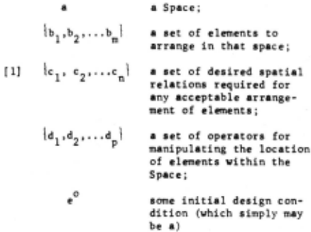
Implicit recognition of the above pro cedure of working has led the designers of all existing computer assisted space planning pro· grams to rely on the following general formula tion. Some of the current programs also facil itate iterative definition and resolution of a problem.
GIVEN:
FIND:
a set of traneformations such that e is generated where
where ~ represents a matching operation.
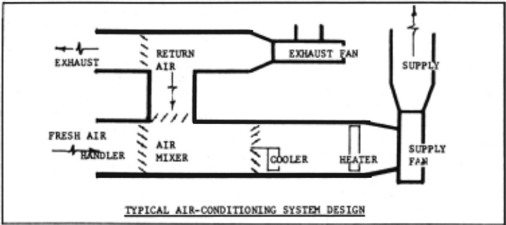
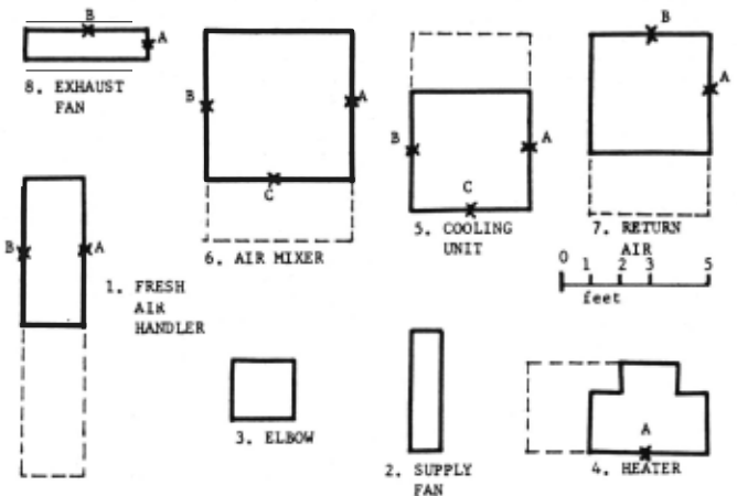
We call this formulation the single level apace planning task. It can depict many typical drafting problems. One example is shown in Figure One. It describes a typical mechanical room layout problem. The elements to be included in the space and the set of relations to be satis
fied are shown at the bottom of the figure.
The Representation of Objects and Relations
The representation of spaces and elements that have been implemented in the various space planning programs all define shape. A major concern has been the accuracy with which shapes are defined. Several are limited to rectangles.~' Some implementations include predicates assigned to domains within the shape to define the type of space being represented. This information is useful for automatically evaluating possible lo cations and eliminating those with overlap con flicts. Usually, only overlaps o£ certain kinds of apaces are allowed. If domain· of apace and their type are included in the ahape representa tion, then the shape can be made up of more than one type of apace, This allows the area adjacent to an element and required for ita uae to be in cluded in its initial shape definition, e.g., the
apace that must remain free behind a desk so that the drawers can be pulled out. Other implementa tions leave the prohibition against certain over laps to be defined by a relation. Several of the space planning implementations also include points that may be defined within a shape (e.g. the location of an electrical outlet) and refer ence can be made to particular sides of objects.
* Of the representations developed to date, Pfeffercorn'a is the most accurate, Hia is likely to be the model for future sophisticated space planning systems (12).
For any particular problem, one can identify a set of relations that should be satis fied if an arrangement is to be accepted. For automatic treatment, the task becomes one of defining a general set of tests with appropriate predicates which are able to depict the wide variety of apecific relations required in any particular class of space planning problems. (Throughout the rest of this paper, we will call such tests Space Relations - or S-Relations.) In the systems implemented to date, S-Relations useful for room arrangement (5), equipment arrangement within a room (1, 12), and building arrangement on a site (6,11), have been con sidered. The set of S-Relations that have been implemented in the GSP space planning program are presented in Table One, ThE task of defining a set of S-Relations that are able to depict the whole aet of space planning tasks, or even a single class of such tasks, remains as a prob
lem for further research.
For ease of description, we say that a S-Relation which has as one of its predicates an element i "belongs" to element i. Most S-Relations implemented in programs thus far act to disqualify certain arrangements of pairs of elements. Thus most S-Relations belong to two elements. (A few belong to a single element, e.g., requiring that the element face southward. The IMAGE system by Johnson et al (6) incorpor ates two S-Relations which belong to three elements,) The reason apace planning is inhe·r ently difficult is the large (potentially in finite) number of location and orientation combinations that are available for any single element. The difficulty involved in evaluating locations for a single element is severely compounded by the interdependencies among elements imposed by the S-Relations. The ex haustive enumeration of all combinations of locations for each element is impractical for
all but the most trivial arrangement problems.
Location Operations
In any space planning program, the types of S-Relations that can be resolved and the char acteristics of the location operators available are intimately related. Let us consider for a moment the kinds of locations that should be gen erated if different S-Relationa are to be satis fied. Almost all S-Relationa that have been in corporated into space planning programs accept either a line of locations (generated along the perimeter of an element, for example) or an area, possibly disjoint, in which any location
~-----~ 0
RE~UIRED RELATIONS
| 1. | Element 2 oriented toward supply. | 8. Point A on element from outside air. 1 <3 |
| 2. | Element 2 <5 from supply Element 3 adjacent to side 3 of | 9. Side 4 on element 7 to side 1 on element adjacent 6. |
| 3. 4. | element 2. Element 3 adjacent to side 2 of | 10. Point B on element 7 <1 point B on element 8. from |
| ·s. | element 4. A on element 4 <1 from | 11. Point B on element 8 from return air. <3 |
| Point point B on element 5. Point A on element 5 <1 from | 12. Side 1 of element 8 toward return air. oriented | |
| 6. 7. | B on element 6. point Point A on element 6 <1 from from point B on element 1. FIGURE ONE- An example of building engineering. | 13. Visibility from door to point c on element 6. planning problem from the area of |
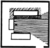
is equally acceptable. For example, the area and line allowed by a SIGHT and an ADJACENT rela· tion are shown in Figure Two. The actual area projected by a S·Relation is only defined if one of the elements it belongs to is located. In the following discussion, we limit consideration to those S·Relations for which an area can be defined. (This important limitation is consider· ed in the final section of this paper.)
S·Relations restricting the locations for an element i will 0 define a set of lines and areas, denoted as si. It is easily 0 proved that the area intersection of any set, Si,can be found by examining only the points of intersection be tween pairs of its areas or lines.t 0 Of course, if two S·Relations belonging to Si define lines which are not parallel, then only the point defined by their intersections need be considered. It ia important to note that it is never necessary to consider location points that are not at the e intersection of two boundaries of areas in S .· 1
In theory, one should be able to project those lines 0 that define the boundaries of the areas in Si and to search their point inter sections for one satisfying all relations. No space planning program has implemented such an approach to locating elements. TWo different approaches have thus far been relied upon.
One approach responds to the interdepend ency of S·Relations and locations by binding them together, one-to-one, much like the recognition and implementation aspects of an interpreter. The IMAGE system, by Johnson et al at M.I.T. (6), starts with an initial (arbitrary) arrangement and upon finding a S·Relation not satisfied, evokes an operator which satisfies it by finding a new location for an element. This approach simplifies the control structure of a apace plan ning system and guarantees that each S·Relation has at least one effective means for responding to it. Its disadvantage is that the operators used are not able to systematically explore the area defined by any s'-Relation. 0 Thus nei.ther the intersection of the area in Si nor any other systematic search of locations can be under taken.** Graaon's program similarly binds S·Relationa to location operators, but incorpor ates operators which generate all locations satisfying a S·Relation (5). Each time an oper ator ia evoked, it produces another location within the area defined 'by its S·Relation. To facilitate search, each S·Relation operator pair is contextually independent. This independence is achieved by restricting the S·Relations that can be represented.
* 0 Conaider the area that is Si. Each of its edges will boundary of one area in will then be defined by the the intersection of be 0 defined by one ~i . Its corners interaection of
two of its edges.
·Eastman (1) and Pfeffercorn (12), on the other hand, keep the binding between S·Relations and location operators loose. In their programs, a limited number of loc.ation operators are pro vided which serve to satisfy whole sets of S·Relations. In Pfeffercorn's DPS program all the possible locations for an element are gen erated in one pass and stored on a list for evaluation. A single location operator gener ates the list and thus it is relied on for satis fying all S·Relations. Eastman's, on the other hand, incorporates operators which sequentially produce locations, one at a time, like Grason's. A set of operators is provided, each producing a different sequence of locations for an element. Thus matching is possible between a set of S Relations belonging to an element and the most appropriate location operator for locating it. In both programs, no one-to-one relation exists and thus each location produced must be eval uated.
In these programs, search of the boundary of the areas defined by different S·Relations is approximated by location operators that re spond to particular arrangement characteristics, e.g., the projected edges of elements and the perimeters of elements. Thus they are usually able to generate some of the locations satisfy ing a set of S·Relations. (The location opera tions are described in more detail later.) The limitation imposed by the approximations used by these programs has not been determined.
Algorithms for Space Planning
TWo alternative but fundamental approaches have been utilized thus far in constructing al gorithms for solving space planning problems. The first takes as its initial step the gener ation and storage of all the possible locations for each individual element. The second step is then to eliminate _all conflicting locations re sulting from overlaps or S·Relations until only
**IMAGE relies on "averaging" the locations pro posed by each S·Relation using a least-squares means-fit procedure. The new location is likely to be different from any of those that are gen erated by the S-Relations (6).
S-RELATIONS :
- (1.) ADJACENT (A, B, SA, 58) - Thil S-Relation apecifiea that element B must have all of ita aide 58 adjacent to aide SA of element A. (A may also be a apace.) Parameters SA and 58 are optional; if one or both are not specified, any aide of the corresponding element may be adjacent;
- SIGHT (A, B, PTA, PTB) - This S-Relation specifies that Point PTA on element A be visible from Point PTB on element B; no aolida may lie in the apace dirently between them. Again, the points are optional and if not defined, all of the element facing the other element must be visible;
- DISTANCE (A, B, F, PTA, PTB) -This 5-Relation defines that Point PTA on element A be less than F units away from Point PTB. on element B. PTA and PTB are both optional parameters. If either or both are omitted, distance is measured from the center of the element;
- ACCESS (A, B, F) - This S-Relation requires that a pathway exist between element A and element B. The pathway must be at least F units wide along its whole length;
- (5 ) ORIENT (A, 8, SA, SB) - This relation orientations between elements 8 and element B must face element A and A must face element B. Either SA both) are optional parameters. defines required A. Side SB of side SA of element or SB (but not
LOCATION OPERATORS :
- SCAN (A, B) - Sequentially generates the complete set of locations for element B, identified by the projection of edges in the space A. (See Figure Three.) It sequentially considers placement of the element in each; all four orientations of the element are considered. SCAN is the most general location operator available in GSP;
- PERIMETER (A, B, SB) - This operator sequentially generates the significant locations for element B along the boundary of a specified and located element in the space, denoted by A. The side SB of element 8 is placed along the common border. One or more calls of thia operator . can satisfy the ADJACENT 5-Relation.
TABLE ONE
Elements of General Space Planner. The above S-Relations and Operators are those implemented in the most current version of GSP.
one or more feasible sets remain, The difficul ties with this approach are (a/ the large amount of memory consumed in storing all location com binations; {b) the large amounts of computer time required to search the combinations; and (c) the strong assumptions that must be made about which locations from among all those pos sible should be stored. Pfeffercorn's program relies on this method to locate single elements. The one effort which totally relied on this ap proach utilized a grid for defining shapes and potential locations (9).*
The second approach, and the one we will ex amine in detail, views the space planning task as one of sequentially generating locations for each element, and adding elements or changing their locations, one at a time, until a single acceptable arrangement is produced. In order that the perturbation of elements to locations not be random, consider them as initially per turbed and evaluated in lexiographic order. The task then is to alter the initial lexio graphic order, using available information, so as to make the search sequence as efficient as possible.
The decisions defining the perturbation se quence and thus the efficiency of space planning in this approach are :
- the sequence of locations considered for a particular element when it is added to the arrangement;
- the sequence in which the elements are added;
- the sequence in which S-Relations are applied to test an arrangement or loca tion and when in the perturbation sequence they are applied;
- when a location operator cannot find a location, or whan a S-Relation is tested and fails, the rule or rules which define what object/location combination is to be perturbed to allow further progress on the problem.
In terms of the formulation represented in eq. [1], this approach relies on operations of the form
- (et, dt+l 1 bt+l) ~ et+l and can be depicted as a search tree.
Of the existing programs for space planning, only two attempt to structure these four decision rules in an efficient manner.** In the following, we present bases on which effic.ient procedures may be developed for responding to the four decision conditions. In most cases, the concepts described have been incorporated in the GSP program now in operation at Carnegie Mellon University. Thus the following can be considered a description of the automated design procedures in GSP. Where the decision rules described have not been implemented, we shall explicitly say so. Also included in the dis cussion is Pfeffercorn's method for treating these four issues. To augment the presentation, the S-Relations and location operators incor porated in GSP are described in Table One. Those interested in a fuller description of GSP should refer to (1, 2).
* Recent contributions in the area of constraint elimination using known alternatives suggest that this approach may still have merit, See (10).
The Sequence of Locations
In the previous discussion of location operations initial consideration was given to the selection of operators and appropriate locations. In the following, we examine more fully rules for sequencing locations.
The basis for selecting a location oper ator and/or location for an element is the inter action between two or more of the S-Relations belonging to the element. If the kinds of S-Relations that are used to specify arrangement objectives are kept very simple, many general izations concerning combinations of S-Relations are possible. For example, suppose adjacency relations require only that any two sides of the elements it belongs to must be in contact. If we also assume that distance relations are always measured from the nearest perimeter of the two objects, then a distance relation of zero is equivalent to an adjacency relation between the aame two elements. In cases wheFe the distance relation is not zero, the locations available to the adjacency relation would be a subset of those defined by the distance relation and could be ignored.
If S-Relations are defined in such a way as to represent the full complexity of meaning ful problems, then the interaction among them cannot be so simply specified. For example, in the S-Relations that have been incorporated in GSP, the DISTANCE S-Relations allows distance between specified points; the ADJACENT S-Relation allows specification of the side to be adjacent. If points and sides are used as references, the relation between the two S-Relations cannot be easily specified. After careful analysis of the interaction of the S-Relations in GSP, the author has concluded that only four warrant special attention in its space planning algo rithms.*
** The breakdown of the remaining programs are as follows : Grason's {5) relies on an exhaust ive search; Negroponte's URBANS (11) operates in the interactive design mode only (? ); and Johnaon's IMAGE (6) relies on a least-squares means-fit procedure for combining S-Relations.
It is not possible in GSP to generate the boundaries of areas defined by S-Relations. GSP relies instead on selecting a location operator that is likely to quickly generate some of the locations in the intersection. It includes an operator that generates locations responsive to the one line producing S-Relation, ADJACENT. It generates locations along the perimeter of a specified or element. Points on the perimeter are selected that are defined by projection of the edges in the current arrangement. See Figure Three. If no ADJACENT S-Relation belongs to the element to be located, a general oper ator called SCAN which tries all corners defined by projections of edges within the space. (See Figure Three.) Pfeffercorn's program relies on one operator similar to SCAN for making all locations.
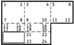
FIGURE THREE - In the twent y-four locations shown, each element would be considered in its four orienta tions. PERI~~TER (in relation to the space ) would generate l-2-3-4-56-12-ll-16-20-22-24-23-17-13-7 in that order.
- The design of S-Relations which can depict the complexities of the real world and which interact in well specified ways is an important research problem. The interactions specially considered in GSP are that ORIENT defines a subcondition of ADJACENT and SIGHT . Only loca tion-orientation combinations which agree with ORIENT need be considered in solving SIGHT. Two ADJACENT S-Relations interact to define one of three conditions : (1 ) a single or possibly two locations; (2) a null location set; (3 ) if the distance between the two elements are the exac t width of the third, a line of locations results . Last, two ORIENTS-Relations belong ing t o the same element must agree, else they de fine a null intersection .
The Seguence of Elements
In general, an efficient space planner is one which can find a feasible arrangement as quickly as possible. An equivalent objective, is to shaw in as few trials as possible that no arrangement is possible.*~' In the following discussion we use this second objective as a substitute of the first .
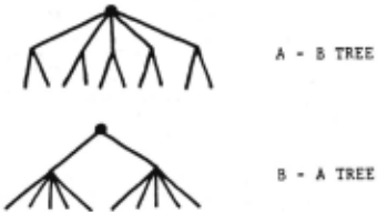
FI�L~E FOUR - Effect of order on the number of operations required to search a tree.
The sequence in which elements are added to an arrangement can significantly effect search efficiency. For instance, consider an arrangement involving two elements, A and B. We ignore consideration of all issues but the number of locations for each element ; element A can be located in five locations, B in two . Two search trees are possible. Both are shown in Figure Four. In order to show that no arrangement is possible, the number of location operations required to search the A-B tree is 15 , while the B-A tree requires 12 . In general, the number of operations required to enumerate the alternating location possibilities of a set of elements, with a fixed number of location
** The relationship between these two objectives may not be obvious . Consider each sequentially genp·ated arrangement of elements as identified by its index n, where 1 < n < N. In order to prove that no arrangement ;ati;fies all 5-Rela tions, all N arrangements must be generated and evaluated . On the other hand, if M arrangements exist that satisfy the S-Relations , their loca tions within the ordering of n can be consid ered random and uniformly distributed (assuming an exhaustive enumeration algorithm) . Thus the average number of locations that must be evaluated is equal to

where M & the number of feasible solutions that exist, M < N. p (x ) corresponds to the accum ulated probabilityn that by the nth draw, one of the M arrangements will be generated . See (14 ) , Chapter 8.
possibilities is equal to W where
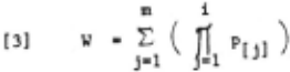
where PJl]' p 121 , ··· p 1 1 is a particular order ing of the locaf1on posWibilities associated with each of the m elements. It is easily proved that W is minimized when elements are added to an arrangement in ascending order of their p. Thus if we can determine the number of potential locations for each element, we can derive the sequence for searching their com binatorial locations most efficiently.*
In reality, no fixed number of locations can be specified for an element; the number changes according to the arrang~ment of the other ele ments. We may approximate the ascending order of p by dynamically evaluating the relative number of locations available after each change in the existing arrangement. After each change, we add to the arrangement next that element with the relatively fewest number of locations avail able to it.
The locations available to an element are those within the intersection of areas and lines defined by each S-delation belonging to that element. These areas can be defined for any S-Relation which has one of its element pred icates already located; for those without one the resulting acceptable area cannot be defined.
We can compute the approximate area for those S-Relations which define them. We can also com bine these areas by assuming that the points in each area are distributed independently of the points in other areas. (Independence is assumed for all but the exceptions listed in the first footnote on the previous page.) We call the total area available to an element i, St. For an unlocated element i there is a set 6 of S-Relations c . , that belong to it. ci denotes the S-Relltions from among the ci which have their other predicate 0 element already located. 6 The set of areas Si identified by ci will define an intersection which is equal to
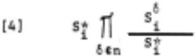
Becauae the size of an element also restricts the number of locations available to it, we divide the area available to locate an element by ita area, or
* In the above, we aaaume that the coat of gen erating locations for all elements is equal. See (13).
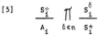
which defines the relative number of disjoint locations available to element i, given the current arrangement.
For each unlocated element, GSP computes the above function and selects the element with the lowest value to locate in the arrangement next,
Pfeffercorn's program includes elements in decreasing order of their size (12). Thus, it approximates the lefthand part of eq. [5].
Sequencing of S-Relations Applied to a Location
Slagle has shown that the most efficient sequence for applying a set of conjunctive boolean tests is to apply them in ascending order of their cost divided by their probability of failing (13). Slagle's results indicate that in testing any location proposed for an element we should base our decision on 8 . , where J

The S-Relations would then be applied in increas ing order of their 8 . Pfeffercorn also lo cates elements in ordJr of their severity, (though he does not state his function for de termining severity) .
In applying the S-Relations to locations, it is useful to distinguish between two types, those that are not affected by the arrangement of elements which are not its predicates, and those that are. An adjacency relation between two elements, no matter how qualified by argu ments, will not be affected by the placement of other elements. On the other hand a aightline relation, defining that an open line of vision must exist between two points or areas, may be affected by any change in the total arrangement of elements. We call the first type of s Relation. local, and the others global. A local S-Relation can be evaluated immediately after placement of the elements which are its pred icates. If it ia satisfied, no later evalua tions are required. Global relations can be affected by any perturbation of the arrangement and thus must be tested after any alteration of the arrangement. In GSP, ADJACENT, ORIE~7A TION, and DISTANCE are local S-Relations.
Backup Procedures .
When a location operator fails to generate an acceptable location for an element, it is due to one of two causes. Either the operator failed to generate a location within an existing inter section of the S-Relation areas, or the inter section of the relevant S-Relations was null. In both GSP and Pfeffercorn's DPS program, the first source of failure is assumed to be negated with careful selection of the location operator. (DPS has only one operator; thus no mistake is possible). Thus any failure is assum ed to be caused by a null intersection.
The likelihood that a 5-Relation will cause failure of a location operator is inversely proportional to the area it defines; the s Relation with the smallest area is thus most critical. One way to resolve failure, then, is to alter the area defined by the most critical $-Relation. If that S-Relation happens to be of the local type, then the~ way to change its area is to alter the location of its prev iously located element. If the S-Relation is global, then moving any one of several elements may alter the $-Relation's acceptable area. ~sp, · in both cases, selects to relocate first the most restrictive element related to the failed one by a local $-Relation. If none is found, then the global S-Relation projecting the smallest acceptable area is considered and its other element selected for re-location. This backup procedure can be applied recursively.
Pfeffercorn's DPS program backtracks by removing both elements of the S-Relation assumed to be most restrictive. It ingeniously composes an arrangement of the two elements that satisfies their $-Relation and attempts to relocate a com posite pair back into the arrangement (12).
Implementation of Constraint Structured Planning in GSP
~SP incorporates no means for directly com puting the area projected by a S-Relation. Thus it cannot take advantage of the location gener ation method outlined in the description of lo cation operations. When considering which ele ment to add next to the arrangements GSP also can only approximate the areas projected by the di fferent S-Relations .
For each $-Relation, GSP has a heuristic function which estimates its allowed area. These estimates make assumptions about shapes (that all are rectangular) and the distribution of elements. They are static, in that they rely on the particular problem definition and not on any particular arrangement . The current form of these estimating functions are presented in Table Two. We expect to improve these methods for estimating areas as our experience with GSP grows.
We have found that incorporation of the pre viously described decision rules is facilitated if the major information they utilize is repre sented in the form of a directed graph, hence the name Constraint Structured Planning. Each element or space defined as part of the problem is represented as a node in the graph. Each S-Relation is represented as one or two directed edges. If a S-Relation belongs to two elements, it defines two edges, one in each direction between them. If a S-Relation is unary or be tween an element and the space, then only one edge is defined. Each edge has a value corres ponding to the area allowed for its successor element when its predecessor element is already located. Each node then takes a 0 - 1 value denoting whether it has been located. For example, the problem shown in Figure One can be represented by the graph shown in Figure Five.
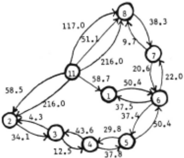
The Constraint Graph depicting any particu lar problem is treated not as an alternative representation of the problem, but as a planning representation that allows anal ysis of import ant characteristics. Thus we use the Constraint Graph in a manner similar to Gelernter's plan ning model for geometry theorem proving (4).
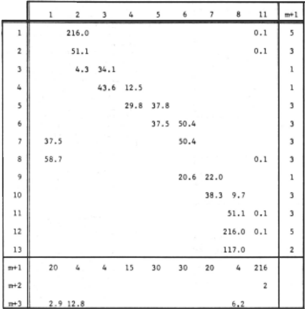
The matrix form of the Constraint Graph is utilized and consists of an edge by node matrix, denoted R(n + 3, m + 1) . The extra rows and columns are used as follows: R(n + 1, i) = the estimated area of element i; R(n + 2, i) denotes whether the element has bpen located antl R (j, m + 1) denotes the type of $-Relation involved. See Figure Six.
On selecting a new element to locate, GSP
In general:
ADJACE!IT:
TABLE 'NO
Current functions for eetimating the area allowed
The area i1 multiplied by the number of orientation·
by an S-Relation . allowed.
c omputes for each element l < i < m the inter section of known areas belonging to it, defined in terms of the estimated disjoint locations allowed, e.g.
Eq. (7] corresponds to eq . [5] .
After an element has been selected and a loca tion proposed, we wish to sequentially evaluate it ac.cording to Slagle's criterion, e.g. eq. [6]. Currentl y , we assume all tests to have the same cost. Thus we make
c 0
m1n
and select largest area of a S-Relation
(belonging to element i) tested
during this iteration.
which
In practice, we apply this algorithm to the constraint graph twice, first subject to the additional constraint that R(j, m + l ) desig nates a local S-Relation, then again without it.
If an element i cannot be located accept ably, the backup procedure is implemented by relocating that element i·', selected from among those where
R(j, i*) > 0 l ~ ~ n. which
[9) min R(j, i).
As above, two iterations may be required, first for local then for global S-Relations.
An Example
Constraint Structured Planning seems to heve FIGURE SEVEN - Example problem and the sequence of alternative states generated by GSP to solve it, powerful capabilities for dealing with a general class of space planning problems. Formal eval uation and empirical testing of its capabilities are currently underway, In order for the reader to better understand the characteristics of its operation, we offer a detailed description of its operation on one trial problem. We use the prob lem presented in Figure One and whose Constraint Graph is shown in Figures Five and Six. We as sign to GSP the problem of arranging the machin ery in Figure One to the space shown in Figure Seven (a), subject to the S-Relations defined in Figure One.
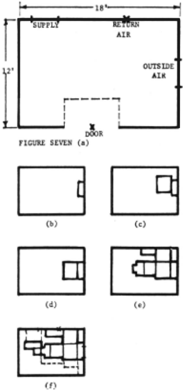
Row n+3 in Figure Six shows the computed intersection areas for the S-Relations upon initiation of the program. Element One is select ed. Locations for it are generated by SCAN, which rotates it and locates it as shown in Figure Seven (6). The intersections of allowed areas (eq. [ 7)) are recomputed for each element. · Ele ment Six is selected next, which is located with SCAN as shown in Figure Seven (c). Of the aix remaining elements, Seven has the smallest allow ed area. Because it must be adjacent to element Six, PERIMETER attempts to locate it but fails to do so for lack of room. The backup algorithm, eq. [9), is initiated and it identifies element Six as the best candidate for relocation. It is moved to the location shown in Figure Seven (d), the. only other acceptable one. Element Seven is then located, followed sequentially by Eight, Five and Four. The result is shown in Figure Seven (e). The last two elements are added, first Three then Eight, after Eight is rotated to satisfy the ORIENT S-Relation, The accepted arrangement is ahown in Figure Seven (f), as printed on our plotter. In preliminary tests, specification, solution, and all plotting for this task took about three and a half minutes of CPU time on Carnegie-Mellon University's IB~l 360/67 computer, using TSS FORTRAN.
Its general performance indicates that Con straint Structured Planning works most efficient ly when the task is highly structured. Search is significantly speeded up if many ADJACE~~ S-Relations are involved. If no S-Relations project areas for unlocated elements, they are chosen according to their approximate size, biggest first. GSP is known to fail on some problems, due to poor handling of global S Relations. Debugging and re-coding are expected to significantly lower current running times.
Conclusion
While Constraint Structured Planning, as implemented in GSP, begins to effectivel y deal with several of the issues inherent in space planning, many remain for more detailed explor ation. Within the problem domain considered here, issues still remain in each of the four decision processes. In the element selection process, only S-Relations which have one of their predicate elements located can currentl y be brought into the analysis, yet the other S-Relations act to delimit allowed areas also. No means has yet allowed us to estimate the re strictions imposed by all S-Relations.
GSP was implemented before the author appre ciated or understood how S-Relations and loca tion operators interact. Thus no means is built into it for projecting areas defined by 5Relations, nor for looking at the boundary intersections between such areas. We anticipate that a system allowing these capabilities would greatly increase the efficiency of search, as well as to allow more varied shapes of elements. Pfeffercorn's method of representation would easily handle these requirements.
Effective backup procedures have been devel oped for treating local 5-Relations, but there has been little progress in characterizing or treating global S-Relations; thev seem to be the cause of most search difficulties.
Future efforts at expanding GSP will include the introduction of variable ahape elements and the appropriate operators and tests to deal with them. We also propose to expand GSP so as to handle hierarchical problem domains, e.g. "arrange the equipment in the rooms, which are arranged and shaped within a building, which is arranged and shaped on a site" (1). Such form ulations clearly open up new problem domains and exciting challenges for future research.
Applications for space planning programs should be obvious. As greater capabilities develop for processing spatial arrangement tasks, better analyzed, better structured, and even more beautiful physical environments should result.
@inproceedings{ijcai1971p3,
  title     = {Heuristic Algorithms for Automated Space Planning},
  author    = {Eastman, Charles M.},
  booktitle = {Proceedings of the Second International Joint Conference on
               Artificial Intelligence, {IJCAI-71}},
  publisher = {International Joint Conferences on Artificial Intelligence},
  editor    = {D.C. Cooper},
  pages     = {27--38},
  year      = {1971},
  url       = {https://ijcai.org/proceedings/1971/3},
}
TY - CPAPER TI - Heuristic Algorithms for Automated Space Planning AU - Eastman, Charles M. T2 - Proceedings of the Second International Joint Conference on Artificial Intelligence, IJCAI-71 PB - International Joint Conferences on Artificial Intelligence PY - 1971 SP - 27 EP - 38 UR - https://ijcai.org/proceedings/1971/3 ER -Copied
Machine-readable versions of this paper, for tools and AI agents:





