Mathematical Models for Automatic Line Detection

MATHEMATICAL MODELS FOR AUTOMATIC LINE DETECTION

Arnold K. Griffith

Artificial Intelligence Laboratory, M.I.T., Cambridge, Massachusetts, U.S.A.

ABSTRACT

The goal of the work here reported Is to Investigate algorithms which find the real straight edges In scenes consisting of prismatic sol Ids, taking Into account smooth variations In Intensity over faces, blurring of edges, and noise. To this end we give In this paper a model of the appearance to an opt leal Input device of such scenes; and describe a sub-optimal statistical decision procedure, based on the model, for the Identification of a 1 lne within a narrow hand on the field of view, given an array of Intensities from within the band.

I. INTRODUCTION

In the following six sections a model­ based 1 lne predicate Is developed analytically. The remaining two sections summarize the results In a computa­ tionally feasible form, and discuss empirical Investigations of Its behavior. The reader may wish to examine these two sections prior to undertaking a study of the analysis upon which the results are based.

I I. THE BASIS OF THE DECISION PROCEDURE Our procedure for determining the ex­ Istence of a real edge within a narrow sub-rectangle on some field of view, given a set of Intensity values J from within the sub-region, Is to compute a probability function of these Inten­ sities, P(CB/J), and to compare this value with a preassigned threshold value. P(CB/J) Is the conditional proba­ bll lty, given that J was obtained over the sub-region, that a boundary 1 lne was actually present and centered In the region. The use of probabll lstlc techniques reflects the assumption that noise prevents us from having access to the set of actual "noise-free" Intensity values, I; over the domain. This proce­ dure can be shown (1, 2) to be optimal In the sense of making the best decision about the existence of a 1 lne In the region over which the Intensity sample J Is taken, given only this Intensity sample, and no spatial context Information about the possible existence of other 1 lnes In the scene, e.g. coter­ mlnal with, or parallel to the line In question. In particular the procedure of accepting the hypothesis of the exis­ tence of an edge when PCCB/J) Is above some threshold has the following proper­ t les:

1. Suppose It Is desired to keep the probability of a false positive error (false claim that a line exists) at or below a certain value. Then there exists a threshold for PCCR/J) which guarantees this hound on the false positive error rate and at the same time minimizes the probability of missing an actual line.
2. Similarly there exists a threshold for P(CB/J) which guarantees a particu­ lar bound on the probabllllty of missing 1 lnes and at the same time gives a minimum rate of false positive errors.
3. Further, there exists a threshold value for PCCB/J) which guarantees that the sum of the probabll I ties of missing a 1 lne and of making a false positive error Is minimized.

The general strategy for establishing a value for P(CB/J) Is based on some simple Bayesian probability analysis. First, we note that by definition:

where CB Is the set of I; 1 s over narrow rectangular domains containing the Image of a centered boundary line. Formula (2.1) follows from the fact that P(CB/J) Is the conditional probability that the actual Intensity pattern over the given sub-region Is some member of CB, given that the pattern J was obtained over the region. It Is thus the sum over all elements of CB, of the con­ ditional probabll lty of this element . being the Intensity pattern, given that the pattern J was obtained. From Bayes' rule we have:

where P(J) Is the a priori probability of occurrence of the obtained Intensity pattern J and P(J, I; ) Is the joint probabll lty of obtaining that pattern along with I; being the real pattern of Intensities. Using this relation, (2.1) becomes:

Clearly P(J), the a priori probability of existence of J, Is the sum of J 1 s joint probabll lty of existence alone with some member of CB, and Its joint probabll lty of existence with a member of CN (the complement of CB In the set Cl · {1;1 ), since this exhausts all possible cases. Hence:

so that (2,2) becomes:

Again, from Bayes' rule liE CN we have:

Thus we can express P(CB/J) as follows:

The remainder of this paper will be devoted to model! lng the set Cl, so as to provide a basts for expressing the various probabll ltles In the above expression. The end result will be a closed form threshold function Q(J) giving an approximate value of P(CB/J) as a function of the set of Intensities contained In the set J.

Ill. DEFINITION AND CATEGORIZATION OF Cl Mathematically the elements of Cl are real valued functions of two variables defined over a narrow rectangular region of the plane. A member li of Cl Is to be thought of as giving the value of the 1 lght Intensity, as a function of posi­ tion, over some narrow rectangular sub region of a two dimensional Image, It should be emphasized that the Intensity functions we have In mind In this sect I on are those glv lng the real Inten­ sities over the sub regions In question, In the absence of any noise and distortion which would be Introduced by some physical Instrument designed to obtain Intensity values. We shall limit out attention to Intensity functions taken over domains of a single preassigned size. It will be apparent that no loss of general! ty wIll result from so doing.

We will define a function to be a member of Cl If It gives the Intensity over some rectangular sub region of a two dimensional Image of some scene having the following properties:

1. The scene consists of prismatic (plane-faced) sol Ids.
2. The Intensity over the faces of the objects, and In the background, Is a smooth continuous function of position.
3. At the Images of the real edges In the scene, the Intensity Is either simply discontinuous In value (hereafter this will be referred to as an 11 edge 11 ); or has an anaomalous value with equal Intensities just to either side, as produced by a crack between blocks or by a highlight. (The latter will heafter be referred to as 11 llnes 11 ).

Further, by assuming that the Inten­ sity values are actually the logarithms of the Intensities In the scene, we have the additional properties:

1. The difference In Intensity across an "edge" will be approximately constant along Its length, although the absolute Intensity along the edge may smoothly vary,
2. The difference between the anomalous Intensity along a "line" and the Intensity of the Immediately surrounding area will be approximately constant along the length of the 1 lne,

Note that the possible existence of shadows need pose no problem, since real edges partially In shadow may be considered for the purposes of the model to be two distinct 11 1 lnes 11 or "edges". Further, the edges of the shadows themselves have properties Identical to those of 11 edges 11 , and may be so modeled.

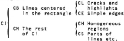
We can be more specific about the previously Indicated division of Cl Into two subsets CB and CN: ·

Let CB be the subset of Cl consisting of all Images of "boundaries", I.e. "lines" or "edges", exactly centered In, and traversing the entire length of, the rectangular domain of definition. An example:

over the rectangle bounded by the points (0,0), (1,0), (0,10) and (1,10),

Let CN be the remainder of Cl.

The class CB may be further subdivided In accordance with the distinction made earl ler between an 11 edge 11 and a 11 1 lne":

>Let CE be the subset of CB consisting of those functions representing simple discontinuities of Intensity. The function given as an example under the definition of CB above Is of this type.

>Let CL be the remainder of CB, I.e. those Intensity functions representing a

1 lne of anomalous Intensity, such as from a high! lght or crack between two blocks. An example:

over the rectangle bounded by the points (0,0), (1,0), (0,10) and (1,10).

Finally we may subdivide the class CN Into two sub-classes:

>Let CH be the subset of CN consisting of Intensity functions over rectangular sub-regions of the plane which are not crossed by Images of any I lnes of the scene. An example:

ICx,y) · .3x + .2y + 10.

over the region bounded by the points (0,0), (1,0), (0,10) and (1,10).

> let CS be the remainder of CN. Intensity functions In this class are those over rectangular sub regions of the plane containing the Image of part of a line, or possibly a closely spaced pair.

The helrarchy of sub categories Just described Is summarized In the following diagram:

IV. NUMERICAL CHARACTERIZATION OF THE MEMBERS OF Cl · AND A PROBABILITY DJSTRIBUTION ON THEM

As a further step In modeling the set Cl, we would 1 Ike to be able to charac­ terize an element of any of the above subsets by some simple numerical description. The functional descriptions given In the above examples are too extensive to lend themselves to the sort of analysis we wish to perform. By way of slmpl lflcaton, we Intend to omit any reference to absolute Intensity, treating, for example, the following two functions:

as eQuivalent, as they differ only by a constant over their domains. Members of CE and CH will thus be characterized only by their "relative amplItudes" or amplItude of discontinuity along their lengths. The above examples are misleadingly simple In that this relative a~pl I tude has been a constant over the whole length of the domain. We actually Intend that there be a small "ripple" In the relative amplitude along the lines, as was lmpl led by the expression "approximately constant" In assumptions 4) and 5) above.

Although we may thus characterize a member of Cl or CE by a nearly constant function of one variable, It Is more practical for the following analysis to assume the domain of definition to be divided Into n approximately square sub components and give a description In terms of then average "relative ampl !­ tudes" over these regions. We propose the notation ICail, ··· , a;n) for a member of Cl, and l(b;J, ··· , b;n) for a member of CE. The function f(x,y), a member of CE, Just referred to would be thus described by the 10-tuple (2, 2, ·· , 2), and would be denoted by 1(2, 2, ··· , 2).

Members of CH are similarly treated, with average gradient within a sQuare sub-region In place of average relative Intensity. For these elments, we will use the notatIon I (C;J , ··· , C;n).

The reader may note that no reference has been made to the remaining class composing Cl, namely CS. Suffice It to say here that In the analysis which follows, such a characterization Is unnecessary, provided one Is wllllhg to trade computational feaslbll lty for a small amount of mathematical exactness. The reader might further be puzzled that no reference Is made In a description of a member of CL or CE to the underlying crosswise gradients to either side of the discontinuity, while members of CH are described entirely In terms of a gradient. The answer Is that In the case of CH, the gradients are the principal effect, whereas In the case of members of CL and CE they are not. In the analysis which follows the gradients In the members ·of CE and CLare Indeed Ignored, since no provision Is made for them In the n-tuple descriptions. However In (1) It Is shown how these can be taken Into acccount to a first order of approximation.

We are now In a position to put a probabll lty distribution on the members of the sets CL, CE and CH based on the above chatracterlzatlon. Specifically, we shall express the a priori probabil­ Ity of existence of a member, e,g, of CL, as a relatively simple function of Ca;1 , ... , a;n ), the n relative amp! I tudes which are used to describe It.

To begin with, assume that each high­ light or crack In scenes under consider­ ation, I.e. each member of CL, has an "Idealized amp! ltude" a. This should be thought of as the relative amplItude which would occur along the whole length of the highlight or crack In the absence of minor Irregularities In lighting or defects In the objects themselves. Let us further assume that the probabll lty distribution P(a) on this parameter Is known, Finally let us assume that for all highlights or cracks with Idealized amplitude a, the various actual relative amplitude values a; 5 are statlstlcallly Independent; and that they have a normal distribution with mean a and standard deviation u Independent of a. From this It follows that the probability P(l(a;1 , .. , a;n)/a)), l,e, the probability of existence of a crack or hlghl lght with actual relative amplitudes a;l, ... a;n along Its length, given that the

Idealized amplitude was a, Is given by:

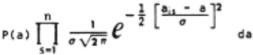
To obtain P( 1Ca;1 , .. , , a;n )), the a priori probabll lty of existence of the highlight or crack with relative ampli­ tudes ail , ... , a;n , we need on! Y sum the above expression over all values of a. Hence for I; a member of CL we have:

Similar formulas hold for members of CE and CH, with b and c In place of a, P' and P" In place of P, and u' and u 11 In place of u,

V. THE PROBABILISTIC RELATIONSHIP BE­ TWEEN AN OBTAINED SET OF INTENSITIES AND A NOISE FREE INTENSITY FUNCTION In this section we shall specify a plausible relationship between obtained

11 nolsy 11 !tensity samples taken over long rectangular regions and actual possible Intensity functions over such regions, I.e. the members of CL, CE and CH. The object will be to give analytic closed form expressions for the values of the conditional probabilities P(J/1; )as apear In the decision predicate (2,4), The relationship between an obtained sample and possible actual Intensity fuctlons Is determined by two effects. The first of these Is the blurring Inherent In any optical system, which turns theoretically sharp Intensity discontinuities Into smooth slopes, and turns hlghl lghts, hypothesized as I Jnes of discontinuity of virtually no width, Into smooth ridges. The second effect Is random time noise.

It will be assumed In what follows that the degree of blurring of edges that Is Inherent In the Intensity samples J obtained by an actual optical Input device from scenes of the sort described Is homogeneous and Isotropic over all scenes under consideration, This assumption might be violated If the scenes had suflclent depth that some parts would be significantly out of focus. However In using the device mentioned In (1) and In the last part of this paper It Is possible to have the optical focus blurring dominated by other blurring effects, which are spatially uniform.

It Is Instructive In considering the relationship between an obtained Inten­ sity sample J and members of CL CE or CH to consider the result of applying this blurring to members of the latter sets. These blurred Intensity functions will be denoted by the symbol 1; 1 · It Is easy to show that If blurring Is uniform and Isotropic over a field of view, It acts on an Intensity function l(x,y) to produce a blurred function I 'Cx,y) as follows:

where B(x,y) Is the Intensity function resulting from applying the blurring to an Intensity function having the value zero except at the origin of the Image space. Now If I; belongs to the class CL then the corresponding blurred version I~ has the property that Its value along any normal to the major axis of the rec­ tangular domain Is given by ag(x) + b, where a Is the relative amplItude of the discontinuity at the point where the normal Intersects the major axis, and g(x) Is related In a simple way to the function B(x,y) just mentioned, It should be emphasized that g(x) Is not dependent on any property of I; other than that It Is a members of CL. Similar results hold for members of CE with a function h(x) In place of g(x); the latter being the Integral of the former. Typical! y g(x) will resemble a "bell curve"; and h(x) a simple step function with rounded corners. The case of members of CH Is similar, but wllh the simple linear function l(x)·mx In place of g(x) or h(x). These properties will be useful later In this section, The geometry over the Image plane of the points at which Intensities are to be obtained has thus far been left unspecified, We will stipulate that this geometry be the same for all of the square sub-regions Into which the rec­ tangular domain of the 1 lne predicate Is divided. In particular we stipulate that It consist of a set of m points lying along a line traversing the square sub­ region through Its center, normal to the major axis of the main rectangular band, The discussion of the "blurred" Inten­ sity functions 1; 1 can now be carried one step farther by cons lderlng the resul·t of restricting these functions to the finite set of points whose geometry has just been described, The resulting In­ tensity function, which we shall denote by the symbol 1;", are clearly formal! y similar to the sets J of obtained Inten­ sity values. The nature of the relationship between these two classes, and Its Implications In developing closed form expressions for the condi­ tional probabilities P(J/1;) will be discussed presently, Meanwhile, various properties of the functions 1," will be noted. First, each consists of n m­ tuples of values, each m-tuple being the value of the corresponding function 1 1 over a set of m points lying along on'e of a set of equally spaced normals to a major axis of the domain of definition of 1,. Secondly, If I; Is In the class CE, CL or CH, then any m-tuple from a corresponding 1:· Is determined entirely from the values of two parameters, and from whether I; came from CL, CE or CH. This follows from the properties of the functIons 1; 1 ment toned In the paragraph before last, and from the uniformity of the geometry of the points In the domain of the function I;"· This may be formally restated as follows: There exists an m·tuple (V 1 , .... , Vm> such that If I (aol , ... , a;n) Is a member of CL, then the corresponding I;" Is given by:

For I; a member of CE there exists a corresponding m-tuple cv,· , .. , v,:, ); and for I; a member of CH an m-tuple (V" , ... , v: ), These m-tuples are slmpl~ the values of the functions g(x), h(x) and l(x) mentioned In the discussion of the functions 1; 1 , suitably scaled,

We now address ourselves to an expression for the value of P(J/1;). This, It may be recalled, Is the condi­ tional probabll lty of obtaining the In­ tensities comprising J, over the region In question, given that the actual In­ tensity over the region Is given by the function I;. If the latter Is a member of CL, CE or CH, then the corresponding I;" as given by (5,1) gives what the values In the set ought to be In the absence of noise. This noise Is assumed to be uniform over the field of view of the Intensity measuring Instrument; and values x of Intensity taken repeatedly at a particular point are assumed to have a distribution around a mean of x given by:

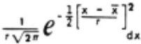
Thus If the sample J Is expressed In the form of n m-tuples, as was lj" In (5.1), by:

then P(J/1;) Is given by:

P(J/1;) · P(J/I(a,,, ... , ain )) ·

This may be expressed In a form similar to (4.1):

VI. TOWARD A CLOSED FORM FOR PCCB/J) In this section we shall show how to express certa~n sums constituting the numerator and denominator of our I lne decision function (2.4) as closed form functions of the Intensity values from a rectangular region. First, let:

and note that P(CB/J) In (2.4) may be expressed In terms of the foregoing as:

It Is the goal of this section to give closed form expressions for the sums CL(J), CE(J), and CH(J) making use of the closed form expressions (4.1), (4.2), (5.3) and (5.4), The matter of the sum CS(J) will be deferred to the next section.

Now (6.1) may be rewritten using (4.1) and (5.3) as:

Because summation of I; over elements of CL Is simply summation over all possible n·tuples of (a; 1 , ... , a;n ), this formula becomes, with a bit of rearranging: CL(J) ·

with, again, F and G given by (4,2) and (5,4) respectively. Also, It Is easy to show that the product over s and the sum over the a;, 1 s may be Interchanged, so that:

As a consequence of Ignoring absolute Intensity we may assume that the obtained Intensities have been normalized by sub regions so that:

and using the definitions:

It Is not difficult to rewrite (5.4) as: G (a is , us 1 ' · · · , u sm ) ·

Combining (6,6) with (~.2) and (6,10):

with b, a~, and R 1 given by (6,7) (6,8) and (6,9). The Inner sum may be put In the form:

which admits of the approximation:

Applying this approximation to the Inner sum In (6,11) we have, after considerable algebra:

where the differentials have been omitted for clarity, This may alternatively be expressed:

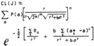
Assuming the Ideal I zed relative amp! 1tudes have a normal distribution, with mean 0 and standard deviation p, then:

where PCCL) Is the a priori probability of a "line". This latter expression for CL(J) may be put Into the form:

Similar formulas exist for CE(J) and CH C J) ·

VI I. RATIONALE FOR IGNORING THE CLASS CS A an analysts similar to the foregoing, with the goal of obtaining a closed form expression for CSCJ), may be avoided. It has been shown In (1) that Q(J) given by:

has the following properties:

1) Q(J) and PCCB/J) are nearly equal when J consists of Intensity values from a narrow region which contains no part of a "boundary", I .e. an edge, hlghl lght or crack. __

2) Q(J) and P(CB/J) are nearly equal when J consists of Intensities from within a narrow rectangular region containing a centered boundary line.

3) Values of Q(J) for J's from various narrow rectangular regions approximately centered on a boundary I lne have a maximum for the set J from a reclon In which the boundary Is exactly centered.

If care Is exercised, Q(J) thus serves as a substitute for PCCB/J). Problems do arise, as the foregoing would predict, when Q(J) Is appl led to Intensity sets from a narrow rectangular band crossed at an ancle of, e.g., 30 decrees by an Intense boundary line. It was necessary In practise to Include a heuristic pro­ cedure for eliminating the spurious line evidence produced by these oblique crosslncs of a region by an Intense boundary. · ·

VIII. SUMMARY: A LINE DETECTION PROCEDURE

The foregolng ·analysls yields a four step procedu,r.e for decldlnc on the exis­ tence of a line between some pair of points on the Image of a scene consist­ Ing of plane faced prismatic sol Ids. The first step Is to make n equally spaced scans across the proposed edge, This yields n m-tuples of Intensity values. The second step Is to compute six values, a;·, R;, a;·', R;'· a·" and R;" from each of these m-tuples. The third step Is to compute from these 6n values the value of:

where the summations are taken from 1·1 to 1·n~ and the six (positive) constants K1, ·· K2' are derivable from the constants In the exponents of (6.12). Finally this value Is compared with a threshold, .and a line Is claimed to exist If the value exceeds lt.

The calculation required to obtain the six values a;·, ... , R;" from an m-tuple of Intensity values Is Quite simple. Consl~er the Intensities obtained from the 1-th scan to be an_m-~ector Q,. Then the·re exist m-vectors V, V' and V" such that:

where · Is the standard dot-product operator. The vectors V, V' and V" are constants, the same for each value of I. Each "R" value Is a 1 lnear combination of a corresponding "a·" value with the dot· product of U, with Itself, I.e., for

The values a,·, R,, ... R,", derived from them successive Intensity values from some short scan across a scene, have a simple Intuitive significance. Recall that they are obtained from (8,2) and (8,3) using three m-tuples of constants symbol tzed as the vectors v, v· and v". Them-tuple of values comprising, e.g., V, are simply them Intensity values which would be obtained from scanning across a perfectly clean paradigm hlgh1 lght by an Intensity measuring device whose blurring characteristics are !dentlcal with the one used In obtaining U,, but which has a negl lglble noise level. Of course the separation of them points Involved In this "paradigm hlgh1 lght profile" must be the same as the actual separation of the points at which the Intensities comprising U;are obtalned._Now suppose that the "para .. lgm profile" V Is least squares fitted to the set of Intensities U;. The factor by which the former must be multlpl led In order to achieve this best fit Is simply so~e constant multiple of ar, We shall thus refer to a value of ar as the "highlight djstlnctness" of the set of Intensities U; from which It was obtained; and refer to the value Qf R; as the "highlight similarity" of U;. It may be shown that a~ has the property of being nei!r zero when the "shape" of the profile U; from which It was computerd Is not at all highlight-like, We may similarly refer tQ a·' as the "edge d I st lnctness" of U; ;' and t2 R 1 as the "edge similarity" Finally V" 's simply a 1 lnearlv Increasing sequence of values; so that a.·" Is a measuer of local gradient 'and R;" a measure of the aparent homogenlty of the 1urface across which the corresponding U; was obtained, It maV be shown that the threshold pro­ cedure Involving (8.1) Is approximately equivalent to the procedure Involving (7.1) and (6.12), The proof of approximate equivalence, which will not be given expl lcltly here, depends on two properties of the latter two expressions. First, If the three terms given by (6.12) are plugged Into (7,1), and the (omitted) mn differentials and mn factors of r, common to all terms, are cancelled; then the resulting coefficients of e are all less than 1, Second, It may be shown C 1) that If the value of (7,1) Is, e.g., above .95, then the two terms of the numerator are necessarily quite unequal. It appears to be necessary to threshold at above this value If the predicate Is to be appl led a large number of times to avoid a significant number of false positive errors.

IX. E11PIRICAL INVESTI�ATIO~IS Investigations of the present 1 lne detection procedure were based on Inten­ sity Information obtained from a computer controlled Image dissector (Information International 11 VIdlssector"). This device makes available to the computer Intensity values from any point on a ~000~ by ~OOO~grld. Intensity values are logarltmlcally scaled with about 80 gray levels for every factor of two In actual Intensity, Several dozen scenes, mostly consisting of plane-faced white prismatic solids, were analysed, with the following conclusions: >VERIFICATION OF UNDERLYING ASSU11PTIONS. It was first necessary to Investigate the val ldlty of various assumptions up on which the foregoing analysis Is based, namely: 1) Intensity values supplied by the Image dissector have an appreciable random noise component which Is Gaus­ sian, and whose level Is Independent both of Intensity and location. 2) Profiles of Intensity along scans normal to real edges In analysed senes are either clIff-shaped or peak-shaped. 3) Various profiles of one or the other of these two types differ only In amp] 1tude, and not In width or skewness. ~) Intensity scans taken normal to a real edge, at regular Intervals along Its length show a rood degree of con­ sistency as to amplItude and type, The first assumption Is theoretically guaranteed by the design of the Image dissector used. Various empirical Inves­ tigations were made which verified this. Assumptions two and three were found to be largely true In that the shape of a~ Intensity profile across a particular edge appeared to be Independent of posi­ tion on the field; and also the shapes of Intensity profiles taken across various highlights or edges between equally lighted uniform faces differed only by multiplicative constants. However, In the scenes ana 1 ysed there appeared to be a larger variety of types of edge profiles than expected, particu­ larly across rather subtle boundaries. A reasonable representative set of six profiles Is Illustrated In figure 2.

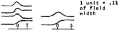
FIgure 2.

Assumption 4 appeared to be true to a marked degree for Intense edges. However this was not always the case for very subtle edges. The lmpl lcatlons of this will be discussed later.

The existence of more than two edge types does not especially Invalidate the foregoing theory and analysts, which may clearly be generalized to six types lnsread of two. This results · In a decision function similar to (8.1) but with the minimum taken over six expressions Instead of two. These six . expressions are calculated usln1 (8.2) and (8.3) and a set of six m-vectors of constants. Each of these vectors Is obtained from one of the profiles of Figure 2, and consists of a set of successive values taken at equally spaced points. The number (m) and spacing will now be discussed.

>�E0~1ETRY OF THE SAI1PL I NG DOMAIN. Two spatially local parameters govern the acquisition of Intensity Information to be given to the present line predicate. These are the length of each of the n sub-scans, and the number (m) of Inten­ sities In each.

It seemed to be of prime lmmportance that the length of the scan be just enough to encompass the entire shape of the various profiles. Referrln1 to figure 2, this would appear to be about 15 units or 1.5~ of the width of the field. If this were much wider, a greater diversity of paradigm profiles would have to be used reflecting various different combinations of gradient values (slopes) of the "tails" of the profiles. Experiments Involving scan lengths of 1'., 2t and 1.5t of the field width confirmed the relative superiority of the latter.

The most Important criterion for estab1 lshlng point separation seemed to be that the spacing be suflclently fine that a scan across a hlghl lght would Include ~t least one value suflclently close to the center of the peak as to have a value within, e.g., 90t of the maximum value at the peak. Referring to Figure 2, the reader may see that the corresponding separation Is one or two units, or about .1t of the field width of the present Instrument. Experiments Involving a spacing of .OSt Indicated no particular advantage over .1t.

For a majority of subsequent experiments values of the (general I zed) threshold function (8.1) and terms thereof, were computed (using (8.2) and (8.3)) from a specific set of 7 16vectors of constants derived from the profiles In figure 2, matched to a spacln1 of .1t of the field width. Intensity values were read at this spacing In sets of 16. The reported results were based on exhaustive calculation of various "R" and "a·" values for scenes of prismatic solids. Typically 100 scans of 500 Intensity values each were made coverln1 the entire scene. For each scan 485 values of each of the 7 "a·"' s and "R' 11 s were computed from each successive 16-tuple of Intensity values. These values were 1raphed or printed line by 1 lne for analysts.

>LOCAL SENSITIVITY. Restricting the function given by (8.1) (or rather the mentioned generalization of It) to a single scan (n · 1) results In a simplified for111ula, since the (a·-a·) 2 terms are all zero. Further, as will be later explained, the a~ terms are of doubtful significance. There thus results a non-linear decision function based on the values of seven "R"'s.

This localized version of the present procedure was compared with two other local edge detection operators. The first operator Is due to Roberts (3) and uses the following function of four In· tensity values v 1 , v 2 , v 3 and v 4 from the corners of a srnall square:

In (1) It was shown that the present edge predicate, even taking Into account Its use of more Intensity values, Is more than twice as sensitive as the Roberts operator. The present operator was also compared with a second difference operator discussed In (4) Involving four successive Intensity valu.es v 1 , v2 , v 3 and v 4 , obtained at equal Intervals along a 1 lne normal to a proposed edge. The formula Is 1lven by:

It may be shown by an argument similar to the one cited In connection with the Roberts operator that the present proce­ dure Is sl lghtly more sensitive In detecting edges than the second difference method provided the latter's point spacing Is wide relative to the blurring. Referlng to the edge profiles at the bottom of figure 2, the reader should note that If these four Intensity values are obtained at 1 unit Intervals around the center of the edge, the value of the operator Is considerably below that which would be obtained If the Intensity values were obtained at, e.g., four unit Intervals. Further If the edge were exactly centered on second or third point, the value of the operator would similarly be reduced. This four value operator thus becomes progersslvly less and less sensitive as the point spacing dereases. This Is true of the Roberts operator as well. On the other hand, In order to avoid missing hlghl lghts, the point spacing should be quite close.

These observations Indicate a marked superiority of the persent procedure In the local detection of edges, etc, provided the cost of obtaining Intensity values Is considerably creater than the cost of computation. In the present Image dissector- computer system this was Indeed the case. Intensity values required an average of one millisecond; whereas the entire time required to calculate a set of 7 11 a· 11 and "R" values from a set of 16 Intensity values was approximately 500 microseconds. In order not to miss highlights, the successive Intensity values In a scan must be obtained at a relatively close spacing. The effective use of a simple second difference operator on such Intensity values would, as cited above, require that e.g., only every fourth Intensity value of the fine scan be used. Its sensitivity would thus be considerably below that of the present operator, which uses all the Intensity values.

>AVERAGE APPARENT DISTINCTNESS. As may be Inferred from the discussion earl ler In this section, the terms In (8.1) Involving the sums over the values a~ and a~' clve an average measure of how distinct an edge or highlight may be fitted to the obtained profiles. These terms seem to be of 1 lttle value In predicting the existence of a real edge or line. Two reasons may explain this. First, large values actually provide necatlve evidence In (8.1) as to the ex­ Istence of an edce or line, reflecting the fact that accordlng to the model very distinct edges are relatively Infrequent. A second problem Is that a very distinct edge crossing the examined region at an oblique angle will produce

a spurious hlch value In this sum. >CONSISTENCY OF EDGE DISTINCTNESS. The seven sums over terms of the form Caf­ a·)2, Caj* 11 -a· 1 ) 2 , etc. In the generalized version of (8.1) have a simple Intuitive slcnlflcance. Consider the sum corresponding to the uppermost profile of flcure 2. This consists of n terms of the form Ca;·-ii*) 2 , where a· Is the average of the n a~'s. Since each ·a· Is a measure of the 11 hlgh11ght ' distinctness" of the scan Intensities from which It was computed, the entire sum gives a measure of the variance of the hlghl lght distinctness along the length of the proposed line. Thus each of the seven terms gives a measure of the consistency of the proposed 1 lne along Its length.

There was Indeed a striking consistency of this sort among the more distinct edges, highlights and cracks, In the many scenes analysed. However, as was pointed out, the more subtle boundaries sometimes showed this consistency, and sometimes not. Since In effect a basic assumption of the model was partially violated, a certain doubt was cast on the validity of these terms. It might be fruitful to use a heuristic procedure which would Increase the 1 lkel I hood of acceptance of a line If this consistency were found; but would have no effect If not. This requires further Invest­ Igation.