
Financial Thought Experiment: A GAN-based Approach to Vast Robust Portfolio Selection
Proceedings of the Twenty-Ninth International Joint Conference on Artificial Intelligence. Special Track on AI in FinTech. Pages 4619-4625.
https://doi.org/10.24963/ijcai.2020/637
Keywords
- Other areas: Financial decision-support system
- Foundation for AI in FinTech: Analyzing highdimentional, sequential and evolving financial data
- AI for trading: AI for novel financial models
- AI for risk and security: AI for financial risk analytics
- AI for trading: AI for portfolio analytics
Abstract
Modern day trading practice resembles a thought experiment, where investors imagine various possibilities of future stock market and invest accordingly. Generative adversarial network (GAN) is highly relevant to this trading practice in two ways. First, GAN generates synthetic data by a neural network that is technically indistinguishable from the reality, which guarantees the reasonableness of the experiment. Second, GAN generates multitudes of fake data, which implements half of the experiment. In this paper, we present a new architecture of GAN and adapt it to portfolio risk minimization problem by adding a regression network to GAN (implementing the second half of the experiment). The new architecture is termed GANr. Battling against two distinctive networks: discriminator and regressor, GANr's generator aims to simulate a stock market that is close to the reality while allow for all possible scenarios. The resulting portfolio resembles a robust portfolio with data-driven ambiguity. Our empirical studies show that GANr portfolio is more resilient to bleak financial scenarios than CLSGAN and LASSO portfolios.
- [Arjovsky et al., 2017] Martin Arjovsky, Soumith Chintala, and Léon Bottou. Wasserstein generative adversarial net- works. In Proceedings of the 34th International Con- ference on Machine Learning (ICML 2017), volume 70, pages 214-223. PMLR, August 2017.
- [Chiu et al., 2017] Mei Choi Chiu, Chi Seng Pun, and Hoi Ying Wong. Big data challenges of high-dimensional continuous-time mean-variance portfolio selection and a remedy. Risk Analysis, 37(8):1532-1549, March 2017.
- [DeMiguel et al., 2009] Victor DeMiguel, Lorenzo Gar- lappi, and Raman Uppal. Optimal versus naive diversifica- tion: How inefficient is the 1/N portfolio strategy? Review of Financial Studies, 22(5):1915-1953, December 2009.
- [Fan et al., 2012] Jianqing Fan, Jingjin Zhang, and Ke Yu. Vast portfolio selection with gross-exposure con- straints. Journal of the American Statistical Association, 107(498):592-606, June 2012.
- [Fouque et al., 2016] Jean-Pierre Fouque, Chi Seng Pun, and Hoi Ying Wong. Portfolio optimization with ambigu- ous correlation and stochastic volatilities. SIAM Journal on Control and Optimization, 54(5):2309-2338, January 2016.
- [Gilboa and Schmeidler, 1989] Itzhak Gilboa and David Schmeidler. Maxmin expected utility with non-unique prior. Journal of Mathematical Economics, 18(2):141- 153, January 1989.
- [Goodfellow et al., 2014] Ian Goodfellow, Jean Pouget- Abadie, Mehdi Mirza, Bing Xu, David Warde-Farley, Sherjil Ozair, Aaron Courville, and Yoshua Bengio. Gen- erative adversarial nets. In Advances in Neural Informa- tion Processing Systems 27 (NIPS 2014), NIPS Proceed- ings, pages 2672-2680. NIPS, December 2014.
- [Hansen et al., 2006] Lars Peter Hansen, Thomas J. Sargent, Gauhar Turmuhambetova, and Noah Williams. Robust control and model misspecification. Journal of Economic Theory, 128(1):45-90, May 2006.
- [Koshiyama et al., 2019] Adriano Koshiyama, Nick Firoozye, and Philip Treleaven. Generative adver- sarial networks for financial trading strategies fine-tuning and combination. arXiv:1901.01751, pages 1-17, March 2019.
- [Mach, 1973] Ernst Mach. On thought experiments. Philo- sophical Forum, 4(3):449-457, 1973.
- [Mao et al., 2017] Xudong Mao, Qing Li, Haoran Xie, Ray- mond Y.K. Lau, Zhen Wang, and Stephen Paul Smol- ley. Least squares generative adversarial networks. In 2017 IEEE International Conference on Computer Vision (ICCV). IEEE, October 2017.
- [Mao et al., 2019] Xudong Mao, Qing Li, Haoran Xie, Ray- mond Yiu Keung Lau, Zhen Wang, and Stephen Paul Smolley. On the effectiveness of least squares generative adversarial networks. IEEE Transactions on Pattern Anal- ysis and Machine Intelligence, 41(12):2947-2960, De- cember 2019.
- [Markowitz, 1952] Harry Markowitz. Portfolio selection. The Journal of Finance, 7(1):77-91, March 1952.
- [Mirza and Osindero, 2014] Mehdi Mirza and Simon Osindero. Conditional generative adversarial nets. arXiv:1411.1784, pages 1-7, November 2014.
- [Pun and Wong, 2015] Chi Seng Pun and Hoi Ying Wong. Robust investment-reinsurance optimization with multi- scale stochastic volatility. Insurance: Mathematics and Economics, 62:245-256, May 2015.
- [Pun and Wong, 2016a] Chi Seng Pun and Hoi Ying Wong. Resolution of degeneracy in Merton's portfolio problem. SIAM Journal on Financial Mathematics, 7(1):786-811, January 2016.
- [Pun and Wong, 2016b] Chi Seng Pun and Hoi Ying Wong. Robust non-zero-sum stochastic differential reinsurance game. Insurance: Mathematics and Economics, 68:169- 177, May 2016.
- [Pun and Wong, 2019] Chi Seng Pun and Hoi Ying Wong. A linear programming model for selection of sparse high- dimensional multiperiod portfolios. European Journal of Operational Research, 273(2):754-771, March 2019.
- [Pun et al., 2016] Chi Seng Pun, Chi Chung Siu, and Hoi Ying Wong. Non-zero-sum reinsurance games subject to ambiguous correlations. Operations Research Letters, 44(5):578-586, September 2016.
- [Pun, 2018a] Chi Seng Pun. G-expected utility maximization with ambiguous equicorrelation. SSRN.com/abstract=3276001, pages 1-23, Decem- ber 2018.
- [Pun, 2018b] Chi Seng Pun. Low-and high-dimensional stock price data (Mendeley data, v3), May 2018.
- [Pun, 2018c] Chi Seng Pun. Robust time-inconsistent stochastic control problems. Automatica, 94:249-257, Au- gust 2018.
- [Srivastava et al., 2014] Nitish Srivastava, Geoffrey Hinton, Alex Krizhevsky, Ilya Sutskever, and Ruslan Salakhutdi- nov. Dropout: A simple way to prevent neural networks from overfitting. Journal of Machine Learning Research, 15:1929-1958, June 2014.
- [Tibshirani, 1996] Robert Tibshirani. Regression shrinkage and selection via the lasso. Journal of the Royal Statistical Society: Series B (Statistical Methodology), 58(1):267- 288, January 1996.
- [Wald, 1945] Abraham Wald. Statistical decision functions which minimize the maximum risk. The Annals of Mathe- matics, 46(2):265, April 1945.
References were extracted automatically from the PDF and may contain errors.
Full text extracted automatically from the PDF; figures, tables and equations may differ. The PDF is the version of record.
1 Introduction
Current trading practice resembles to Ernst Mach's thought experiment in the sense that traders leverage their own perceptions of the future stock market and invest accordingly. A good trader should be able to perceive multiple market scenarios that are close to the reality and aim to construct a portfolio that performwell under all those imaginary conditions. Such a thinking process is a typical thought experiment, where by conceiving "good copies of facts" and employing "method of variation", we can "discover new properties" and establish new theory; see [Mach, 1973].
By drawing connections between portfolio construction and thought experiment processes, we naturally turn to the state-of-the-art machine learning technique: generative adversarial networks (GAN). When it was first introduced by
∗Contact Author
[Goodfellow et al., 2014], GAN was used to generate samples that are indistinguishable from the real data by a discriminating neural network. Many developments of GAN have been made to make the generated sample more alike to the reality and promote the diversity of generated output; see [Mirza and Osindero, 2014; Arjovsky et al., 2017; Mao et al., 2017]. The application of GAN to financial strategies has a potential to objectively and computationally replicate the thought experiment for portfolio construction. Recently, [Koshiyama et al., 2019] adopted conditional GAN, a variation of GAN, for fine-tuning financial trading strategies. The application of GAN was proved to be advantageous over conventional techniques in some cases. However, our application of GAN has very different objectives and thus requires an innovative architecture.
The most vivid illustration of GAN application in finance may be through an analogy to image generation, for which GAN was initially devised. Imagine that the returns of the stocks in the market on each day is a line of an "artwork" and the nature continues painting it from left to right. We have the access of the semi-finished paining up to date. To experiment the financial thoughts, we ought to draft the next few lines and plan accordingly from the big picture. GAN has the capacity of drafting the next few lines based on what have been painted. In this paper, we extend the framework of GAN such that it can conduct the financial experiment for portfolio construction at the same time. Our proposed framework adds a regressor on top of the existing discriminator and generator in GAN, for which we termed as GAN with regessor or GANr in short.
To design a GAN architecture for financial applications, we incorporate the financial knowledge in empirical finance into GANr. Due to the stationarity consideration, we use only the daily financial data of recent past one year as training data, leading to small sample size. Thanks to the introduction of gross-exposure constraints, our proposed framework, GANr, is still applicable for the market with arbitrarily many risky assets. Following [Fan et al., 2012], we recast the classical portfolio risk minimization problem with gross-exposure constraints as a regression problem with a ℓ1-norm constraint, which can be considered as a simple neural network and be embedded into the GAN framework. Heuristically, the generator of GANr still aims to deceive the discriminator. On the other hand, the major difference between GANr and the original GAN is that the generator of GANr will also maximize the risk of the portfolio. Such a proposal resembles the theories of the worst-case utility and robust controls; see [Wald, 1945; Gilboa and Schmeidler, 1989; Hansen et al., 2006]. Robust portfolio selection has been studied extensively in the literature on financial mathematics; see [Fouque et al., 2016; Pun and Wong, 2015; Pun et al., 2016; Pun and Wong, 2016b; Pun, 2018c; Pun, 2018a]. However, most of their ambiguity sets are model-based and none of them can handle arbitrarily many risky assets. With the power of neural networks and the idea of GAN, we study the vast robust portfolio selection problem computationally.
The rest of the paper is organized as follows. Section 2 describes some of the major developments about GAN, on which we heavily rely for our proposed GAN architecture. In Section 3, we propose and describe in detail a new GAN structure and apply it to a risk minimization problem. The new GAN architecture is examined with empirical data and the test results are summarized in Section 4. Section 5 concludes.
2 Related GANArchitectures
2.1 GAN
GAN, originated by [Goodfellow et al., 2014], consists of two competing networks: generator (G) and discriminator (D). The former takes in latent noise (z) to simulate the fake data. The generated fake data along with some real data are then input to the latter, which estimates the probability of the input data being real. In this process, generator aims to minimize log(1 - D(G(z))) while discriminator maximizes its binary cross entropy, where D(x; θD) is a scalar multi-layer perception (MLP) function with parameters θD representing the probability that x came from the data rather than the generator's distribution and G(z; θG) is another differentiable MLP function with latent input z and parameters θG that outputs a fake data of the same dimension of the real data. The interaction between G and D mathematically amounts to a minmax game:
where for GAN, the value function V takes the form:
in which, pz(z) is the prior on the latent noise z. Training D and G are equivalent to determining θD and θG.
2.2 Conditional GAN (CGAN)
Since the introduction of the GAN, many improvements on GAN have been made. One of them is conditioning both generator and discriminator on some auxiliary information y; see [Mirza and Osindero, 2014]. Specifically, conditional GAN (CGAN) feed the auxiliary information y about the intended output into the generator on top of the latent noise. Then, the auxiliary information y along with the generated data are input to the discriminator. Mathematically, the value function in (1) for the CGAN takes the following form instead:
The slight modification of the networks is simple but yet powerful. Not only does CGAN improve the quality of the generated image "categorically" as demonstrated in its original paper, but is also adopted by [Koshiyama et al., 2019] for financial trading strategies and outperforms other traditional techniques in numerous cases. Moreover, the conditioning property in CGAN is desired in applying a GAN-based approach in regression problems.
2.3 Least Squares GAN (LSGAN)
When GAN was first introduced, [Goodfellow et al., 2014] acknowledged that in practice, GAN may experience vanishing gradients. To alleviate this issue, [Mao et al., 2017] proposed a different loss function for the minmax game between the generator and discriminator. The novel reformulation of GAN is named least squares GAN or LSGAN in short. Instead of using the sigmoid cross entropy as the loss function, the discriminator of LSGAN measures the difference between the output and the real label, which are quantified. When the output is more deviated from the real label, the model is penalized more. The new formulation generates more gradients to update the generator and stabilizes the training process. Moreover, LSGAN incentivizes generator to simulate outputs that are close to the decision boundary of the discriminator, ensuring that the fake data does not lie too far away from the decision boundary, a problem that GAN suffers intrinsically.
Suppose we use the a-b coding scheme for the discriminator, where a and b are the labels for fake data and real data, respectively. LSGAN trains D and G by solving the minimization problems iteratively:
where c denotes the value that G wants D to believe for fake data. The benefits and effectiveness of LSGAN are documented in [Mao et al., 2019].
Conditional LSGAN (CLSGAN)
It is noteworthy that the idea of conditioning in the CGAN can be incorporated into LSGAN, for which we call it as conditional LSGAN (CLSGAN). For simplicity, we label the real and fake data by 1 and 0, respectively. Then, the value functions of the discriminator and the generator with conditioning on the auxiliary information y become
The 0-1 coding scheme suffices for our application as we will introduce a scaling factor in our new GAN architecture that will absorb the belief on fake data generation. The CLSGAN is interesting in its own right while it serves as a building block of our proposed GAN architecture.
3 GANwith Regressor (GANr)
In this paper, we present a new GAN architecture, namely GAN with regressor (GANr), whose design is motivated by robust portfolio construction while its applicability is extendable to general regression problems with robustness. Its generator and discriminator closely follow the architecture of CLSGAN in pursuit of good data simulation. Therefore, GANr preserves the merits of CGAN and LSGAN. In addition to generator and discriminator networks, GANr contains the third neural network, regressor (R), which solves some regression problem of our interest. The graphical illustration of GANr architecture is presented in Figure 1.
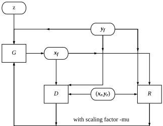
In GANr, the auxiliary information y is taken as the response (dependent variable) while x is the features (independent variables). We use R(x; θR) to represent the regression model, parameterized by θR, for the paired data (x, y) such that y = R(x; θR) + ϵ. Similarly, training R is equivalent to determining θR. Mathematically, the value functions of GANr are defined as follows:
where µ > 0 is a tuning parameter balancing the impacts of D and R on G and g : R+ → R+ is a transfer function, for which we take g(·) = tanh(·) in our numerical studies. It is found necessary to introduce the transfer function because scales of discrimination loss and regression loss are very different, which may lead to a generator disregarding the reality of generated data in pursuit of a huge reduction in regression loss. Hence, the transfer function can limit the impact of regressor on the generator's loss.
It is clear that when µ = 0, GANr is reduced to CLSGAN.
The financial interpretation of the parameter µ will be discussed later. As illustrated in Figure 1, D and R are trained simultaneously and then the results are feedback for training G. Since D and R are mathematically similar, it is easy to see that GANr enjoys the same computational advantages of LSGAN, while the idea of conditioning, borrowed from CGAN, guarantees the stability of the GANr's performance.
Different from the initial objective of GAN, the primary objective of GANr is to solve for the regressor R, which is referred to as financial solution. The original components of GAN, D and G, are trained to simulate different realistic scenarios for the agent (i.e. investor in financial applications). Then the R is trained to perform well in different scenarios, by noting that its training involves both real and different fake data. The feedback from R to G ensures that the G is aware of how the R performs and generates tougher scenarios, which makes an essential difference from "generating fake data and then performing regression with a bunch of fake data separately" (that corresponds to the case µ = 0). The R resulted from GANr will be more resilient to bleak scenarios.
3.1 Application to Vast Portfolio Selection
In this section, we illustrate the application of GANr to vast portfolio selection. Suppose that the market consists of p stocks with returns, r = (r1, r2, . . . , rp)′ for the future one period (for which we consider one day in this paper). Based on the modern portfolio theory, initiated in [Markowitz, 1952], we presume that an investor aims to determine her portfolio, characterized by a weight vector w with w′1 = 1, by minimizing the risk (variance) of the daily return of her portfolio: Var(w′ r), subject to the gross-exposure constraint |w|1 ≤ c. Since the gross-exposure constraint is introduced, we can consider a large universe of stock market with p even larger than n, the training sample size. Following [Fan et al., 2012], we recast the vast portfolio selection as a regression problem by noting that
where y = rp and xj = rp - rj for j = 1, . . . , p - 1. Therefore, the construction of gross-exposure-constrained minimum variance portfolio can be converted into the following regression problem:
where x = (x1, x2, . . . , xp-1)′ . When we apply GANr to vast portfolio selection, we substitute the regression loss function in (3) by (4). The rest of implementation follows the procedure stated in the previous section or Figure 1. Finally, we output the minimizer of R which suggests a trading strategy.
It is important to note that the problem (4) is an approximation to the minimum variance problem as the regression outcome depends on the choice of y. When y is properly chosen, the portfolio is nearly optimal. There are some proposals stated in [Fan et al., 2012], while the authors pointed out that
(4) is equivalent to the problem of using the "assets" with returns x to track y. Therefore, we pick equally weighted (EW) portfolio as y in our paper as it is free of model assumption and performs well out-of-sample in terms of Sharpe ratio and many measures; see [DeMiguel et al., 2009]. In other words, we specify the pth asset as the EW portfolio of the rest p - 1 assets and note that p could be arbitrary.
In finance, EW portfolio can represent the overall performance of the market. The implementation of GANr is based on conditioning on y and thus the GANr's simulation of multiple scenarios is conditional on the market's performance and the generator yields the artificial data of excess returns of the stocks with respect to the market. These financial insights, which are in line with the market's practice, explain the rationale behind incorporating the conditioning into GANr.
3.2 Relation to Robust Portfolio Selection
The benchmark portfolio selection problem (4) can be considered as a special case of (3) when there is no fake data (generation). Hence, it is interesting to heuristically explore what the add-ons by GANr bring to the portfolio selection.
From R's perspective, D is not directly involved in R's minimization but impacts it through regulating G. The probabilistic interpretation of the regression loss function in (3) can be through an alternative measure QG for real and fake data that is characterized by the current generator G: V [R] GANr (R) = EQG [(y - (w∗ )′x - b)2 ]. Let us denote the measure for real data only by P, which is the measure used in (4). In every iteration of (3), V [R] GAN (R) uses different measure QG. Note that the existence of D is to ensure that G generates the data close to real data. Hence, we can define a set of measures using the mathematical notations: Q := {QG|G is regulated by D in the fashion of CLSGAN}. An important observation is that the V [G] GANr (G) in (3) is adversarial to R since a negative scaled transferred regression loss is part of the generator's loss function. Hence, the equilibrium of GANr will find the worst-case measure among Q for R. Heuristically, in equilibrium, GANr solves a robust control version of the portfolio selection problem (4):
The similar minimax problems have appeared in many studies on robust controls or robust portfolio selection; see [Hansen et al., 2006; Wald, 1945; Fouque et al., 2016; Pun and Wong, 2015; Pun et al., 2016; Pun and Wong, 2016b; Pun, 2018c; Pun, 2018a]. However, the unique features of GANr are its applicability to a large universe of stocks and its characterization of purely data-driven ambiguity set.
Economically speaking, using the real data for solving (4) implicitly assumes that the future market movement replicates the history, which may not be advocated by many market practitioners. Hence, it makes perfect sense to conduct thought experiment on various future scenarios that are inferred with the historical data. The trading strategy resulting fromGANr resembles the outcome of thought experiment on vast robust portfolio selection.
µ in GANr
Now, the user-defined parameter µ in GANr can be interpreted as the ambiguity aversion level of the investor. When µ is of a small value, the generator tends to generate data closer to the real data, which implies that the investor believes that the real data are good enough to reflect the future market situation. When µ is large, the generator tends to generate more severe market scenario, where even minimum variance strategy has a relatively large variance. As a rule of thumb, µ should be set a small value during the boom period and a large value during the recession period.
4 Empirical Studies
4.1 Data andMethodology
We examine GANr with two empirical datasets on S&P 500 index components (p = 408) for two different periods, namely the recession period from 1 December 2006 to 30 June 2009 and the boom period from 31 December 2015 to 29 December 2017. The data can be downloaded from [Pun, 2018b]. For each of the dataset, we examine the outof-sample performance of LASSO (see [Fan et al., 2012]), GANr (with µ = 0.1, 0.2 in (3)) and CLSGAN (with µ = 0 in (3)) portfolios.
The daily returns of the recent past one year are used as training set, allowing generator and discriminator to learn about the distribution of real daily returns conditional on the EWportfolio's return. The regressor simultaneously take into account both real and fake data, learning a robust minimum variance portfolio. As the regressor basically does LASSO regression (see [Tibshirani, 1996]), the selection of tuning parameter λ is determined by cross-validation with the first training set and sticks with it throughout the study. Specifically, the first training set is divided into 12 folds. In each fold, the chronological order of the data is maintained. Then we carry out 12 folds of cross-validation tests to determine the optimal λ with the highest portfolio return. Such crossvalidation approach has been carried out in [Pun and Wong, 2016a; Chiu et al., 2017; Pun and Wong, 2019] and yields desirable outcomes.
4.2 Configuration of GANr
In our empirical studies, the generator consists of five layers (including input and output layers) and each layer has p nodes. Specifically, the first two hidden layers adopt ReLU activation function with dropout (see [Srivastava et al., 2014]), where the dropout rate is 0.25, and the last two layers (including output layer) use tanh activation function without dropout. As for the discriminator, the three hidden layers are identical to the generator's, while its output layer uses a linear activation function with one output node. The regressor has no hidden layer and uses a linear activation function with one output node and ℓ1 kernel regularizer.
The latent noise input follows a uniform distribution while the daily EW portfolio return fed into the generator is resampled with replacement from the real daily EW portfolio return. Though the latent noise is completely random, GANr may still run into mode collapse problem. Therefore, the weights of all layers in GANr are initialized with standard normal distribution.
Two important parameters in training GANr are the number of epochs and the number of discriminator training cycles per an update of generator. Our empirical studies are conducted in a moving window fashion and thus for the first test, we train GANr 10000 times (i.e. 10000 epochs). Note that subsequently, only one day of new return data is added and the oldest day of data is removed. By assuming that the distribution of daily returns does not change drastically, we reduce the number of epochs to 150 and initialize the networks weights with the optimal weights from the previous day, starting from the second training of GANr. The discriminator and regressor are trained 5 times every training of generator. The batch size is 50. This approximately corresponds to the number of working days in one financial year. In [Mao et al., 2017], it is found that RMSProp optimizer exhibits more stable performance than Adam. Hence, we adopt RMSProp for the back-propagation. The learning rate is set at 0.0001.
4.3 Empirical Results
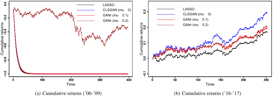
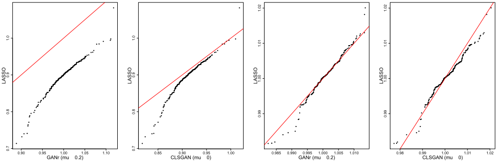
The empirical results are presented in Figures 2 and 3 and Table 1, where the LASSO portfolio serves as a benchmark. Figure 2 presents the time-series plot of the cumulative outof-sample returns of the portfolios. Figure 3 provides the QQ plots of the out-of-sample returns of the GAN-based portfolio and the LASSO portfolio over different periods. Table 1 presents the statistics of the portfolios, including risk (measured by the (annualized) volatility of the daily portfolio returns), portfolio Sharpe ratio, and five quantile values of the daily portfolio returns.
Robustness of GANr Portfolio
Figure 2(a) shows that except for the GANr (µ = 0.2), the other three portfolios perform bad during the recession period. Even the GANr (µ = 0.2) also suffers loss, it is clear that it has better protection when the market is volatile, which echoes our initiative on setting a large µ during the recession. In the Figure 2(b) for the boom period, two GANr portfolios with µ = 0.1 and µ = 0.2 perform similarly. At the first glance, CLSGAN performs the best in terms of return but we should also examine the variance and quantile statistics to investigate their risk profiles. Both Figures 2(a) and 2(b) show that GAN-based portfolios improve the LASSO portfolio.
Figures 3(a) and 3(b) show that the two GAN-based portfolios not only uniformly outperform the LASSO portfolio over the period from 2006 to 2009, but also demonstrate a robustness against bleak stock market. Both GANr and CLSGAN portfolios beat the LASSO portfolio at almost all quantiles as shown by the fact that almost every point lies on the right hand side of the identity line in Figures 3(a) and 3(b). Moreover, at lower quantiles, the points are further from the identity line. Thus, over the recession period, LASSO suffers a more severe loss than the two GAN-based portfolios.
The GANr portfolio demonstrates a more robust performance than the CLSGAN portfolio over two test periods. In terms of downside risk performance, CLSGAN is slightly worse off as compared to LASSO. As depicted in 3(d), LASSO returns consistently defeats that of CLSGAN over the return range from 0.99 to 1.00, while the comparison between the two portfolios over the return range from 0.98 to 0.99 is inconclusive. In contrast, GANr almost unanimously outperforms LASSO at all extremely low quantiles while having a comparable return level to LASSO at all other quantiles.
Both empirical results indicate that by subjecting portfolio construction to a more volatile market (with a GAN-based approach), the portfolio becomes more robust to bear market.
Improvement on Risk and Sharpe Ratio
For the recession period, the performance of GANr (µ = 0.1) and CLSGAN are almost identical, while GANr (µ = 0.2) performs the best. All of them successfully bring down the annualized volatility of the LASSO portfolio. They also beat LASSO portfolio at all five quantiles of annual returns. At lower quantiles, the difference is more significant than that at higher quantiles as shown in Table 1, Figures 3(a) and 3(b).
For 2016-2017 data, GANr outperforms CLSGAN and LASSO in terms of annualized risk. The low volatility of GANr is attributed to the robustness of the GANr portfolio. CLSGAN performs the best in terms of Sharpe ratio. Table 1 suggests that CLSGAN yields the highest annualized return thanks to its high-performing upside gains (q0.5, q0.75 and q0.9). It is further confirmed by Figures 3(c) and 3(d). The former shows that GANr and LASSO have comparable performances at higher quantiles. In comparison, Figure 3(d) depicts that CLSGAN tend to perform better than LASSO at higher quantiles of annualized return.
5 Conclusion and Future Research
This paper presents a way of financial thought experiment with the aid of the GAN framework. We illustrate the thought experiment with vast robust portfolio selection. Our proposed framework is, however, extendable for general regression problems. By providing another angle of view on GAN, we link the proposed GANr with the robust control/optimization theory. In particular, the design of the GANr architecture is perfect for financial applications, where we need to simulate multiple complex scenarios. An noteworthy merit of GANr is that it allows users to control the trade-off between the closeness to real data and the volatility of the generated data with tuning parameter µ. Not only does GANr simulate data, but also helps users find a robust portfolio that is resilient to bleak financial market. As shown by our empirical studies, GANr portfolio consistently outperforms CLSGAN and LASSO portfolios in terms of the lower quantiles.
Some promising future research include incorporating GANr with other GAN architectures, such as Wasserstein GAN (see [Arjovsky et al., 2017]) or generalizing the mean squares loss function in the regressor network to any utility or loss function. It will also be interesting to explore the mathematical property of GANr, such as its relation to Pearson χ2 divergence as in [Mao et al., 2017].
Acknowledgements
Chi Seng Pun gratefully acknowledges Nanyang Technological University, Start-up Grant (No.: 04INS000248C230) and Ministry of Education (Singapore), AcRF Tier 2 grant (Ref. No.: MOE2017-T2-1-044) for the funding of this research.
| Year | Strategy | Risk | Sharpe ratio | q0.1 | q0.25 | q0.5 | q0.75 | q0.9 |
|---|---|---|---|---|---|---|---|---|
| '06-'09 | LASSO | 0.5941 | - | 0.8595 | 0.8849 | 0.9014 | 0.9138 | 0.9343 |
| CLSGAN (µ = 0) | 0.4006 | - | 0.8843 | 0.8992 | 0.9120 | 0.9230 | 0.9413 | |
| GANr (µ = 0.1) | 0.4006 | - | 0.8843 | 0.8993 | 0.9120 | 0.9230 | 0.9413 | |
| GANr (µ = 0.2) | 0.4748 | - | 0.9677 | 0.9855 | 1.0000 | 1.0131 | 1.0328 | |
| '16-'17 | LASSO | 0.0902 | 1.7511 | 0.9946 | 0.9977 | 1.0006 | 1.0037 | 1.0079 |
| CLSGAN (µ = 0) | 0.1066 | 2.4279 | 0.9934 | 0.9967 | 1.0008 | 1.0046 | 1.0093 | |
| GANr (µ = 0.1) | 0.0878 | 2.0172 | 0.9944 | 0.9973 | 1.0004 | 1.0037 | 1.0079 | |
| GANr (µ = 0.2) | 0.0791 | 2.3592 | 0.9949 | 0.9978 | 1.0005 | 1.0035 | 1.0071 |
Table 1: Annualized risk (volatility), Sharpe ratio, and different quanitles of daily returns for four portfolios. The Sharpe ratios over the recession period ('06-'09) are negative for all portfolios and thus they are not reported as a negative Sharpe ratio lacks of interpretability.
@inproceedings{ijcai2020p637,
  title     = {Financial Thought Experiment: A GAN-based Approach to Vast Robust Portfolio Selection},
  author    = {Pun, Chi Seng and Wang, Lei and Wong, Hoi Ying},
  booktitle = {Proceedings of the Twenty-Ninth International Joint Conference on
               Artificial Intelligence, {IJCAI-20}},
  publisher = {International Joint Conferences on Artificial Intelligence Organization},
  editor    = {Christian Bessiere},
  pages     = {4619--4625},
  year      = {2020},
  month     = {7},
  note      = {Special Track on AI in FinTech},
  doi       = {10.24963/ijcai.2020/637},
  url       = {https://doi.org/10.24963/ijcai.2020/637},
}
TY - CPAPER TI - Financial Thought Experiment: A GAN-based Approach to Vast Robust Portfolio Selection AU - Pun, Chi Seng AU - Wang, Lei AU - Wong, Hoi Ying T2 - Proceedings of the Twenty-Ninth International Joint Conference on Artificial Intelligence, IJCAI-20 PB - International Joint Conferences on Artificial Intelligence Organization PY - 2020 SP - 4619 EP - 4625 DO - 10.24963/ijcai.2020/637 UR - https://doi.org/10.24963/ijcai.2020/637 ER -Copied
Machine-readable versions of this paper, for tools and AI agents:





