
Towards Alleviating Traffic Congestion: Optimal Route Planning for Massive-Scale Trips
Proceedings of the Twenty-Ninth International Joint Conference on Artificial Intelligence. Main track. Pages 3400-3406.
https://doi.org/10.24963/ijcai.2020/470
Keywords
- Planning and Scheduling: Real-time Planning
- Multidisciplinary Topics and Applications: Databases
- Planning and Scheduling: Planning Algorithms
- Multidisciplinary Topics and Applications: Transportation
Abstract
We investigate the problem of optimal route planning for massive-scale trips: Given a traffic-aware road network and a set of trip queries Q, we aim to find a route for each trip such that the global travel time cost for all queries in Q is minimized. Our problem is designed for a range of applications such as traffic-flow management, route planning and congestion prevention in rush hours. The exact algorithm bears exponential time complexity and is computationally prohibitive for application scenarios in dynamic traffic networks. To address the challenge, we propose a greedy algorithm and an epsilon-refining algorithm. Extensive experiments offer insight into the accuracy and efficiency of our proposed algorithms.
- [Babak et al., 2018] Javani Babak, Babazadeh Abbas, and Ceder Avishai (Avi). Path-based capacity-restrained dy- namic traffic assignment algorithm. Transportmetrica B: Transport Dynamics, pages 1-24, 2018.
- [Cai et al., 1997] X. Cai, Ton Kloks, and C. K. Wong. Time- varying shortest path problems with constraints. Networks, 29(3):141-150, 1997.
- [Cao et al., 2012] Xin Cao, Lisi Chen, Gao Cong, and Xiaokui Xiao. Keyword-aware optimal route search. PVLDB, 5(11):1136-1147, 2012.
- [Chen et al., 2019] Lisi Chen, Shuo Shang, Christian S. Jensen, Bin Yao, Zhiwei Zhang, and Ling Shao. Effec- tive and efficient reuse of past travel behavior for route recommendation. In KDD, pages 488-498, 2019.
- [Chen et al., 2020a] Lisi Chen, Shuo Shang, and Tao Guo. Real-time route search by locations. In AAAI, 2020.
- [Chen et al., 2020b] Lisi Chen, Shuo Shang, Bin Yao, and Jing Li. Pay your trip for traffic congestion: Dynamic pric- ing in traffic-aware road networks. In AAAI, 2020.
- [Dafermos and C., 1972] Dafermos and Stella C. The traf- fic assignment problem for multiclass-user transportation networks. Transportation Science, 6(1):73-87, 1972.
- [Dafermos and Sparrow, 1969] Stella C. Dafermos and Fred- erick T. Sparrow. The traffic assignment problem for a general network. National Bureau of Standardsb-, 1969.
- [Dijkstra, 1959] Edsger Wybe. Dijkstra. A note on two prob- lems in connexion with graphs. Numerische Mathematik, 1:269-271, 1959.
- [Ding et al., 2008] Bolin Ding, Jeffrey Xu Yu, and Lu Qin. Finding time-dependent shortest paths over large graphs. In EDBT, 2008.
- [Dotoli et al., 2014] Mariagrazia Dotoli, Slim Hammadi, Karama Jeribi, Carmine Russo, and Hayfa Zgaya. A multi-agent decision support system for optimization of co-modal transportation route planning services. In CDC, 2014.
- [Dumitrescu and Boland, 2003] Irina Dumitrescu and Natashia Boland. Improved preprocessing, labeling and scaling algorithms for the weight-constrained shortest path problem. Networks, 42(3):135-153, 2003.
- [Huang et al., 2017] Wei Huang, Chunwang Yan, Jinsong Wang, and Wei Wang. A time-delay neural network for solving time-dependent shortest path problem. Neural Netw, 90:21-28, 2017.
- [Levin et al., 2010] Roy Levin, Yaron Kanza, Eliyahu Safra, and Yehoshua Sagiv. Interactive route search in the pres- ence of order constraints. PVLDB, 3(1):117-128, 2010.
- [Li et al., 2007] Qing Li Qing Li, Guangjun Liu Guangjun Liu, Wei Zhang Wei Zhang, Cailu Zhao Cailu Zhao, Yixin Yin Yixin Yin, and Zhiliang Wang Zhiliang Wang. A spe- cific genetic algorithm for optimum path planning in intel- ligent transportation system. In ITST, 2007.
- [Li et al., 2013] Jing Li, Yin David Yang, and Nikos Mamoulis. Optimal route queries with arbitrary order con- straints. IEEE Trans. Knowl. Data Eng., 25(5):1097-1110, 2013.
- [Liang and Wang, 2018] Hongwei Liang and Ke Wang. Top- k route search through submodularity modeling of recur- rent POI features. In SIGIR, pages 545-554, 2018.
- [Liebig et al., 2017] Thomas Liebig, Nico Piatkowski, Christian Bockermann, and Katharina Morik. Dynamic route planning with real-time traffic predictions. Inf. Syst., 64:258-265, 2017.
- [Lim and Rus, 2012] Sejoon Lim and Daniela Rus. Stochas- tic distributed multi-agent planning and applications to traffic. ICRA, pages 2873-2879, 2012.
- [Lim et al., 2009] Sejoon Lim, Hari Balakrishnan, David Gifford, Samuel Madden, and Daniela Rus. Stochastic motion planning and applications to traffic. The Interna- tional Journal of Robotics Research, 2009.
- [Nikolova, 2006] Evdokia Nikolova. Optimal route planning under uncertainty. In ICAPS, 2006. [Peeta and Mahmassani, 1995]
- Srinivas Peeta and Hani S. Mahmassani. System optimal and user equilibrium time- dependent traffic assignment in congested networks. An- nals of Operations Research, 60(1):81-113, 1995.
- [Shang et al., 2013a] Shuo Shang, Lu Hua, Torben Bach Pedersen, and Xike Xie. Finding traffic-aware fastest paths in spatial networks. In SSTD, 2013.
- [Shang et al., 2013b] Shuo Shang, Lu Hua, Torben Bach Pedersen, and Xike Xie. Modeling of traffic-aware travel time in spatial networks. In MDM, 2013.
- [Shang et al., 2015] Shuo Shang, Jiajun Liu, Kai Zheng, Hua Lu, Torben Bach Pedersen, and Ji-Rong Wen. Plan- ning unobstructed paths in traffic-aware spatial networks. GeoInformatica, 19(4):723-746, 2015.
- [Shang et al., 2016] Shuo Shang, Danhuai Guo, Jiajun Liu, and Ji Rong Wen. Prediction-based unobstructed route planning. Neurocomputing, 213(NOV.12):147-154, 2016.
- [Sharifzadeh et al., 2008] Mehdi Sharifzadeh, Moham- mad R. Kolahdouzan, and Cyrus Shahabi. The optimal sequenced route query. VLDB J., 17(4):765-787, 2008.
- [Wang and Ran, 2012] Xuren Wang and Chunfeng Ran. Dy- namic path planning algorithm based on time-dependent road network. In Congress on Intelligent Systems, 2012.
- [Xu et al., 2017] Ying Xu, Lisi Chen, Bin Yao, Shuo Shang, Shunzhi Zhu, Kai Zheng, and Fang Li. Location-based top-k term querying over sliding window. In WISE, pages 299-314, 2017.
- [Zeng et al., 2015] Yifeng Zeng, Xuefeng Chen, Xin Cao, Shengchao Qin, Marc Cavazza, and Yanping Xiang. Op- timal route search with the coverage of users' preferences. In IJCAI, pages 2118-2124, 2015. IJCAI
References were extracted automatically from the PDF and may contain errors.
Full text extracted automatically from the PDF; figures, tables and equations may differ. The PDF is the version of record.
1 Introduction
With the continued development of GPS-enabled devices (e.g., vehicle navigation systems and smart phones) and online map-based services (e.g., Google Maps), route search and planning have attracted significant attention in recent years (e.g., [Dumitrescu and Boland, 2003; Sharifzadeh et al., 2008; Levin et al., 2010; Shang et al., 2013b; Li et al., 2013; Zeng et al., 2015; Liang and Wang, 2018; Xu et al., 2017]). Some studies on this topic aim to generate a route based on an optimization goal (e.g., shortest distance, minimum travel time) under user-defined constraints (e.g., source and destination) over traffic-aware road networks [Cao et al., 2012; Shang et al., 2013a; Shang et al., 2015; Liebig et al., 2017; Shang et al., 2016].
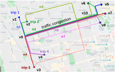
However, these studies find an optimal route only for a single trip query. As online map-based services are becoming increasingly popular, it is not uncommon that a great number of users may issue trip queries simultaneously or within a short period of time, especially during rush hours. In such case, recommending the optimal route based on each individual query may induce potential traffic congestion. Let us consider Figure 1 as an example. Let trips 1-4 be four trip queries that are issued simultaneously. Each trip query consists of a source (marked with a circle) and a destination (marked with a diamond). Vertices v1, v2, v3, and v4 are the sources of trips 1-4. Vertices v5, v6, v7, and v8 are the destinations of trips 14. Routes π1, π2, π4, and π6 are optimal travel routes for trip queries 1-4, respectively. We see that all optimal routes will travel between vertices v9 and v10, which may lead to traffic congestion. In turn, the congestion may delay the travel times of all routes that cover the segment between v9 and v10.
∗Corresponding author
Consequently, given a large number of trip queries issued simultaneously, we need to regard these queries as a whole and generate a route planning for each query such that the global travel time for all queries is minimized. In particular, we can adjust the optimal routes of trip 2, trip 3, and trip 4 to π3, π5, and π7, respectively. Even if they are sub-optimal results for individual queries, traffic congestion between v9 and v10 can be alleviated and the global travel time of all trips 1-4 is improved.
In this light, we study a novel Global Optimal Route (GOR) problem: Given a traffic-aware road network and a set of trip query Q, we generate a travel route for each query such that the sum of travel times for all queries is minimized. In our settings, travel time of each edge depends on both the edge's minimum travel time and flow of vehicles, the query finds a route combination (set of routes) such
that global travel time is minimized. The GOR problem has
a broad range of application, including traffic management,
route planning and congestion alleviation. By processing all
trip queries issued within a short period of time in a batch
mode, we are able to reduce the average travel time and avoid
traffic congestion, especially during commute hours and holidays. The problem is challenging due to its high computational cost. The time complexity of our straightforward exact algorithm is exponential to the number of queries. As a result, it is impossible to find the optimal solution in interaction time. To answer the problem efficiently, we first propose a greedy algorithm. Based on the greedy algorithm, an ϵ-refining algorithm and corresponding pruning techniques are developed to further decrease the global travel time effectively. Based on our experimental results, our proposal is capable of achieving high efficiency and high efficacy when processing 10,000 trip queries simultaneously.
Related work. A host of studies were developed to answer optimal route queries under different settings [Nikolova, 2006; Li et al., 2007; Ding et al., 2008; Lim et al., 2009; Shang et al., 2013a; Chen et al., 2020a; Chen et al., 2020b; Chen et al., 2019]. These studies only consider the optimization of individual route query. Existing studies of trafficbased global optimization problems [Dafermos and Sparrow, 1969; Dafermos and C., 1972; Lim and Rus, 2012; Dotoli et al., 2014; Babak et al., 2018] can be regarded as the flow assignment problem rather than real-time route planning problem, where the routes are pre-defined and they search for an optimal flow assignment to each route. The queries proposed by these studies are based on a singe trip. Hence, their solutions cannot be used to answer our problem. Additionally, time-dependent road network [Peeta and Mahmassani, 1995; Cai et al., 1997; Ding et al., 2008; Wang and Ran, 2012; Huang et al., 2017] is a representative dynamic network, where each edge has different weight at different time, while in our work the weight (travel time) depends on the real-time flow, thus the optimization methods cannot be used in our problem. To the best of our knowledge, none of the existing algorithms can address our problem as they either target a single query or target different settings.
2 Preliminaries and Problem Statement
Traffic-aware road networks. We define a traffic-aware road network by a connected and directed graph G(V, E, tm), which consists of a set of vertices V representing road intersections and a set of edges E representing road segments. Each edge e(vi, vj) ∈ E connects two end-points vi and vj where vi, vj ∈ V . Function tm : E ↦→ R assigns a realvalued weight tm(e)1 to edge e that denotes the minimum travel time on road segment e (i.e., the travel time of e when there are no vehicles).
Traffic flow. In this paper, traffic flow is defined as the number of vehicles on an edge e at a particular time t, denoted by fe, is computed by Equation 1.
Here, fe ′ (t) denotes the number of non-query vehicles on edge e at time t while fe ′′ (t) is the number of vehicles using our query system. Note that how to compute fe ′ (t) is beyond the scope of this paper, and the solutions we proposed are independent of the initial traffic and the original number of vehicles that traverse the segment but do not use the query system.
1 For ease of presentation, we use e to represent e(vi, vj) where the context is clear.
Time-flow function. The time-flow function is used to compute actual travel time of an edge if we take into account the traffic flow. Following existing studies [Lim and Rus, 2012; Babak et al., 2018], we use two popular time-flow functions (cf. Equations 2 and 3) to computer the actual travel time of segment e, which is denoted by t(e).
Here, fe denotes the number of vehicles on segment e, α, σ, ϕ, and β are road-specific parameters, which are determined by segment attributes (e.g., speed limit, road width). Note that our proposal is independent of the values of these parameters. How to set appropriate values for these parameters is beyond the scope of our study.
Route and travel time. A route π is defined by a finite sequence of vertices 〈v1, v2, . . . , vk〉. Denoted by T(π) the actual travel time of π is the sum of actual travel times of each road segment in π (cf. Equation 4). Similarly, the minimum travel time of a route π, denoted by Tm(π), is the sum of minimum travel times of each road segment in π (cf. Equation 5).
Problem definition. Given a traffic-aware road network G(V,E, tm) and a set of trip queries Q = {q1, q2, . . . , qn} where each query qi = {si, di, τi} consists of a source location si, a destination location di, and a departure time τi, the Global Optimal Route (GOR) problem finds an optimal route πi from si to di for each trip qi ∈ Q such that the global travel time for the route combination Π (i.e., Π = {π1, π2, ..., πn}) is minimized. Note that the global travel time of Π, denoted by GT(Π), is computed by Equation 6.
3 Solutions for GOR Problem
3.1 Exact Algorithm
Given a GOR query Q, a straightforward method is to evaluate all possible route combinations and select the combination that has the minimum global travel time. Specifically, for each trip query qi ∈ Q we run Depth-First Search (DFS) on the road network to find all possible routes from si to di. Here, we employ a pruning technique [Shang et al., 2015] that enables early termination of DFS. Next, for each route combination we compute its exact global travel time. We return the route combination with the minimum global travel time as the result.
Complexity analysis. The exact algorithm evaluates every route combination. Assume that the number of possible routes of a trip is p and the number of vertices of each route is |π|. The total number of route combinations is p|Q| and we need to visit |π||Q| vertices to compute the global travel time of each route combination. For each vertex, we have to traverse each qi ∈ Q to count current flow on the edge. Hence, the time complexity of exact algorithm is O(p|Q| |π||Q|2 ).
3.2 Greedy Algorithm
From Section 3.1 we see that the exact algorithm is computationally prohibitive for answering the GOR problem when |Q| is large. Hence, a greedy algorithm is proposed to answer the GOR problem efficiently. The high-level idea is to generate a global optimal route for each trip query qi ∈ Q concurrently through network expansion.
Route label. To enable concurrent network expansion of routes, we maintain a route label l(qi) = 〈va, τa, πa〉 for each trip query qi that records its evaluation progress. The label l(qi) consists of three elements: va, currently arrived vertex; τa, the time arriving at va; πa, the up-to-date route from qi.s to va. Initially, the currently arrived vertex for each trip query qi is the source location and arrival time is the departure time of qi (i.e., τi).
Network expansion strategy. Given a route label l(qi) = 〈va, τa, πa〉, we select an optimal subsequent vertex based on network expansion. In particular, we select an adjacent vertex vj of va that has the minimum estimated global travel time. Here, the estimated global travel time for route label l(qi), denoted by EGT(l(qi)), is computed by Equation 7.
Algorithm details. Algorithm 1 presents the pseudo code of our greedy algorithm. Initially, we initialize our route combination set Π and priority queue H that sorts trip queries in ascending order based on l(q).τa (line 1). Then we insert all initial route labels of trip queries from Q to H (lines 25). During the search and update process, in each iteration we select a route label l(q) from H and expand its route to next vertex until H is empty, namely all trip queries are processed to destinations (lines 6-25). To be specific, each time we get the l(q) with minimum l(q).τa on the top of H (line 7), for currently arrived vertex l(q).va, we select one of its adjacent vertices v with minimum EGT(l′ (q)) for expansion (lines 8-18). For each adjacent vertex we check whether it conflicts two thresholds: it cannot appear twice in the trip's planned route l(q).πa and its minimum travel time to destination d cannot be larger than that of l(q).va (line 10). If it satisfies both thresholds, we compute the traffic flow for the edge e(l(q).va, v) and the expected travel time EGT(l′ (q)) (lines 11-12). In the next, if EGT(l′ (q)) is the currently minimum, we update l′ (q).τa and l′′ (q) is used to store the l′ (q) with minimum EGT(l′ (q)) (lines 13-16). Once the greedy selection is completed, l(q) has to be updated (line 19). At the end of each iteration, if the trip query is processed to its destination d, we add l(q).πa to Π, else we insert the up-to-date l(q) into H again waiting for next expansion (lines 20-24).
Algorithm 1 Greedy Algorithm
Input: Traffic-aware road network G(V, E, tm); A set of trip queries Q = {q1, q2, . . . , qn}; Output: A route combination Π = {π1, π2, ...π|Q|};
1: H ← ∅; Π← ∅; 2: for each trip query qi in Q do 3: Initialize l(qi); 4: H.push(l(qi)); 5: end for 6: while H ̸= ∅ do 7: l(q) ← H.pop(); 8: for each adjacent vertex v of l(q).va do 9: l′ (q) ← 〈v, l(q).τa, l(q).πa.add(v)〉; 10: if v /∈ l(q).πa and tm(v, d) < tm(l(q).va, d) then 11: Compute the traffic flow on edge e(l(q).va, v); 12: Compute EGT(l′ (q)); 13: if EGT(l′ (q)) is the minimum then 14: l′ (q).τa ← l(q).τa + t(e(l(q).va, v)) 15: l′′ (q) ← l′ (q) 16: end if 17: end if 18: end for 19: l(q) ← l′′ (q) 20: if l(q).va == d then 21: Π.add( l(q).πa); 22: else 23: H.push(l(q)); 24: end if 25: end while 26: return Π3.3 ϵ-Refining Algorithm
To improve the result quality, we develop an ϵ-refining algorithm that refines the route combination generated by our greedy algorithm. The high-level idea works as follows: After generating the result route combination Π, we perform a particular refining operation, including add, drop, and swap, on each route if the operation can decrease the global travel time of Π at least by a factor of 1 + ϵ. Specifically, for each route πi ∈ Π we select a refining operation that produces the maximum decrease of global travel time and check if it is improved by a factor of 1 + ϵ (i.e., GT(Π) GT(Π′ ) is no less than (1+ϵ) where Π′ denotes the route combination after performing the selected refining operation).
Refining Operations
We detail three refining operations: add, drop, and swap. The ϵ-refining algorithm reuses the results of greedy algorithm and refines each route π ∈ Π from the source vertex. We evaluate each route sequence of π (i.e., ∀(vi-1, vi, vi+1) ∈ π where i ∈ [1, |π| - 1]) and perform the following refining operations if possible.
- drop (vi): drop a vertex vi ∈ π if |π| >3 and an edge exists between vi-1 and vi+1.
- add (v): add a vertex v ∈ (V \π) to π if v is an intermediate vertex between vi and vi+1.
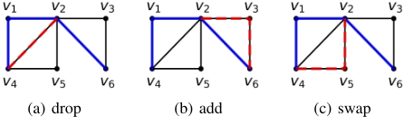
- swap (vi, v): swap a vertex vi ∈ π with another vertex v ∈ (V \ π) if more than one alternative intermediate vertices exist between vi-1 and vi+1.
Figure 2 exemplifies drop, add, and swap operations. The blue edges are the primitive route π = 〈v4, v1, v2, v6〉 generated by the greedy algorithm. The red edges in Figures 2(a), 2(b), and 2(c), are the refined segments after performing drop, add, and swap operations, respectively.
Consider the drop operation in Figure 2(a), if an edge between v4 and v2 exists, the decrease of global travel time is ∆GTdrop = t(e(v4, v1)) + t(e(v1, v2)) + t(e(v4, v1))′ + t(e(v1, v2))′ - t(e(v4, v2)) -t(e(v4, v2))′ , where the front part is the reduced travel time of e(v4, v1) and e(v1, v2), and the latter is the increased travel time of e(v4, v2), t(·) denotes the changed travel time of the adjusting trip while t(·)′ denotes the changed travel time of other trips that are influenced by the refinement. For the add operation in Figure 2(b), where v3 can link v2 and v6 as an intermediate vertex, if we adjust the route using v3, the decrease of global travel time is ∆GTadd = t(e(v2, v6)) + t(e(v2, v6))′ - t(e(v2, v3))- t(e(v2, v3))′ - t(e(v3, v6)) -t(e(v3, v6))′ . For swap operation in Figure 2(c), where v5 can take place of v1 as an intermediate vertex linking v4 and v2, if we adjust the route using v5, the decrease of global travel time is ∆GTswap = t(e(v4, v1)) + t(e(v4, v1))′ + t(e(v1, v2)) + t(e(v1, v2))′ - t(e(v4, v5)) - t(e(v4, v5))′ - t(e(v5, v2)) - t(e(v5, v2))′ .
However, in order to update the travel time of each trip, we need to compute the current flows of all altered edges each time we perform a refining operation, which is very timeconsuming. To improve the efficiency of refining operations, we develop pruning strategy for each type of operation by computing the corresponding upper bound of decreased travel time. In particular, the upper bounds of decreased travel time for drop, add, and swap, denoted by UBdrop, UBadd, and UBswap, respectively, are computed as follows.
Thus, for each operation we first compute UB(i.e., UBdrop, UBadd, and UBswap) to determine whether the operation is valid. If UB cannot decrease the global travel time by a factor of 1+ϵ (i.e., GT/(GT-UB) ≤ 1+ϵ), the operation
Algorithm 2 ϵ-Refining Algorithm
Input: Traffic-aware road network G(V, E, tm); Output: A refined route combination Π′ ;A route combination Π = {π1, π2, ...π|Q|}; Parameter ϵ; 1: Init: Let H = ∅; 2: for each trip query qi in Q do 3: Initialize l(qi); 4: H.push(qi); 5: end for 6: while H ̸= ∅ do 7: q ←H.pop(); 8: compute ∆GT of each valid operation; 9: select the operation with maximum∆GT; 10: if GT GT-∆GT > (1 + ϵ) then 11: GT←GT-∆GT; 12: update the route label l(q); 13: update q′ s route in Π; 14: end if 15: if l(q) isn't adjusted to destination then 16: H.push(l(q)); 17: end if 18: end while 19: return Π′is invalid, else we further compute the exact decreased global travel time ∆GT (i.e., ∆GTdrop, ∆GTadd, and ∆GTswap) to compare with other operations.
Algorithm details. Algorithm 2 presents the pseudo code of our ϵ-refining algorithm. The query input includes a trafficaware road network G(V, E, tm) and the results of greedy algorithm, a refining factor ϵ is selected as parameter, while the output is the refined route combination. Initially, we maintain a dynamic priority heap H for selecting the route label l(q) with minimum l(q).τa (line 1). Then, we insert all initial route labels of trip queries from Q to H based on l(q).τa (lines 2-5). During the refining process, we apply a valid operation with maximum decrease of global travel time to update global travel time and corresponding route labels. The process terminates when no new operation is valid to produce a better result, namely all routes' adjusting progresses are finished (lines 6-18). To be specific, in each iteration, we select the route label l(q) on the top of H (line 7). Consider the current route sequence of l(q).va, we compute the corresponding upper bound of decreased travel time first to determine whether the operation is valid. If an operation is valid, we further compute the exact decrease (line 8). After selecting the operation with the maximum global travel time decreased (line 9), we apply the operation with maximum decrease to update global travel time GT, the route label l(q) and corresponding route in Π respectively if the global travel time is improved at least by a factor of 1+α (lines 10-14). At the end of each adjustment, if l(q) is adjusted to its destination, it doesn't need to be refined any more, else we insert up-to-date l(q) into H again for next adjustment. Finally, we return the refined Π as the result, denoted by Π′ .
Complexity analysis. AssumeGT0 is the global travel time of the obtained results of greedy algorithm and GT ′ is the global optimal travel time. By utilizing the small constant ϵ, the maximum number of operations in ϵ-refining algorithm m depends on the ratio of GT0 to GT ′ . The value of m is computed as follows.
To find a valid operation, we check all cases of drop, add, and swap operations in each adjustment. The time complexity is O((n11 + n12 + n13)|Q|) + O((n21 + n22 + n23)|Q|)+O((n31+n32+n33+n34)|Q|) = O(|Q|2 ). Here, n11,n12,...,n34 are the number of other influenced trips on altered edges and they are up to |Q|. Assume the maximum number of vertices of all routes is k and the number of influenced trips by this adjustment is n, then updating routes and progress records requires time complexity O(kn). Here, m is a constant. Thus, the time complexity of the ϵ-refining algorithm is O(mkn|Q|2 ) = O(|Q|3 ) for k is much smaller than |Q| and n is up to |Q|.
4 Experimental Study
4.1 Experimental Settings
Compared algorithms. We study the performance of the following proposed algorithms: the greedy algorithm (Section 3.2) and the ϵ-refining algorithm (Section 3.3). And to evaluate the result quality of the two algorithms, we implement an individual-based search algorithm. Specifically, given a set of trip queries Q, for each query qi ∈ Q we derive a route π with the minimum travel time (i.e., Tm(π)). Note that the exact algorithm requires at least 1 day with default setting, thus we do not report its performance. In remaining parts of this paper, the greedy algorithm is denoted by "Gre-Alg.", the ϵ-refining algorithm is denoted by "RefAlg.", and the individual-based search algorithm is denoted by "Ind-Alg.".
Data and queries. We use two road networks in our experimental study, namely San Joaquin County Road Network (TG) 2 and the New York Road Network (NYN) 3 , which contain 18,263 vertices and 23,874 edges, and 95,581 vertices and 260,855 edges, respectively. The road networks are maintained by memory-based adjacency lists. We pre-compute the all-pair minimum Tm(Π) using Dijsktra's algorithm [Dijkstra, 1959] and store the results on disk. All algorithms are implemented in Java and tested on a Windows 10 platform with Intel(R) Core(TM) i5-9300H Processor (2.40 GHz) and 16GB memory. The sources and destinations are selected randomly. The departure time of each trip is randomly generated within a specific time range. The main performance metrics are CPU time and the global travel time (GT). Unless stated otherwise, the experimental results are averaged over 20 independent trials with different query inputs. We apply Equation 2 (cf. Section 2) as time-flow function by default. The default parameter settings are listed in Table 1.
2 https://www.cs.utah.edu/∼lifeifei/SpatialDataset.htm
3 https://publish.illinois.edu/dbwork/open-data/
| TG | NYN | |
|---|---|---|
| Number of trip queries |Q| | 2,000-10,000 /default 10,000 | 4,000-20,000 /default 10,000 |
| Refining factor ϵ | 0.02-0.10 /default 0.02 | 0.02-0.10 /default 0.02 |
| α (Equation 2) | 0.02-0.10 /default 0.02 | 0.02-0.10 /default 0.02 |
| σ (Equation 3) | 0.15 | 0.15 |
| ϕ (Equation 3) | 20-100 /default 20 | 20-100 /default 20 |
| β (Equation 3) | 2 | 2 |
4.2 Experimental Results
Effect of query trip count. First, we investigate the effect of the query trip count |Q| on the performance of the algorithms with the default setting. Intuitively, a larger |Q| causes more vertices to be processed (being selected or being adjusted). Thus, a larger |Q| leads to more computation effort and the CPU time cost is higher for all algorithms. Additionally, a larger |Q| leads to the increment of traffic flows on edges, and thus increases the travel time. In this case, Gre-Alg and Ref-Alg may reduce the global travel time substantially. Figure 3 shows the CPU time and the global travel time of the results of three algorithms in TG and NYN respectively. As expected, when |Q| becomes larger, the CPU time increases for all algorithms. Compare with Ind-Alg, the GreAlg performs slightly slower. We also find that Ref-Alg requires more CPU time than the other two algorithms due to its update operations in each iteration of refinement. Nevertheless, we can see all algorithms are reasonably efficient. It is clear that the route combination generated by Gre-Alg consistently exhibits less global travel time compared with Ind-Alg. Compared with Ind-Alg, Ref-Alg greatly decreases the global travel time. It is worth noting that there are little traffic flow on each edge when |Q| is small, in this case the improvements of Gre-Alg and Ref-Alg are negligible (i.e., |Q|=2,000). This is because that the performance when traffic flow is large as |Q| increased, the improvement of Gre-Alg and Ref-Alg is significant (i.e., Gre-Alg can reduce over 30% global travel time and Ref-Alg can reduce over 60% global travel time compared with Ind-Alg when |Q| is 20,000 in NYN). These results demonstrate that Gre-Alg and Ref-Alg are effective to alleviate traffic congestion, especially when |Q| is large.
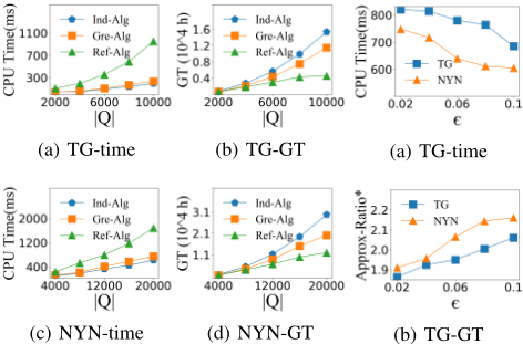
Figure 4: Effect of ϵ
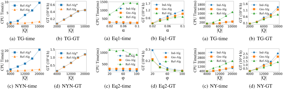
Figure 6: Effect of ce
Figure 7: Worst-Case Measurement
Effect of ϵ. Figure 4 shows the efficiency and efficacy performance as we vary ϵ. The total number of operations is inversely proportional to the value of ϵ (cf. Section 3.3). Intuitively, a larger ϵ means fewer valid operations, thus less CPU time is required. However, a larger ϵ also results in more global travel time. The minimum global travel time, denoted by GT∗, is the global time of individual optimum when we assume that fe = 0. Though the global optimal travel time GT ′ is unobtainable, GT∗ can take place of GT ′ to compute an approximation ratio upper bound for GT∗ is close to GT ′ . The upper bound of the approximation ratio, denoted by "Approx-Ratio*", is the ratio of GT to GT∗. Thus, the value of "Approx-Ratio*" is larger than that of actual approximation ratio for GT∗ is smaller than GT ′ .
Effect of pruning techniques. We study the effect of pruning techniques in Ref-Alg . The Ref-Alg without pruning techniques is denoted by "Ref-Alg*". In Figure 5, With the help of pruning techniques, the performance of Ref-Alg is improved by about an order of magnitude when |Q| is large (i.e. |Q| ≥10,000). And as expected, Ref-Alg* only reduce little global travel time compared with Ref-Alg. These results demonstrate the accuracy of our proposed pruning rules.
Effect of time-flow functions. To study the scalability of our proposed algorithms, we apply two different time-flow functions in Section 2 (Equations 2 and 3) and vary the corresponding parameters. Intuitively, a larger value of α and a smaller value of ϕ will cause more congestion for increased actual travel time, and the CPU time will increase accordingly. Due to space limit, we only show the results in TG. Figure 6 illustrates the CPU time and global travel time of the three algorithms when we apply Equation 2 and Equation 3 as our time-flow functions, respectively. It is clear that CPU time increases as we increase α or decrease ϕ as shown in Figure 6(a) and Figure 6(c), respectively. In Figure 6(b), when we vary α from 0.02 to 0.10, an increasing trend regarding global travel time is observed for all methods. However, the increasing trend of Ref-Alg is less significant than the other two methods, demonstrating the stronger capability of Ref-Alg in alleviating traffic congestion and reducing the global travel time. In Figure 6(d), when we vary ϕ from 20 to 100 in Equation 3, the global travel time decreases. The results demonstrate that our proposed algorithms are capable for handling the query for most of settings, and different time-flow functions allow our proposed algorithms to apply to diverse traffic models.
Worst-Case measurement. The worst-case measurement is the worst experimental result with the default setting among 20 independent experiments. Figure 7 reports worstcase measurements. We observe that Gre-Alg and Ref-Alg are both able to compute the query in interaction time. Generally, the CPU time is at most 1,200 ms in TG and 2,400 ms in NYN, respectively. Additionally, Ref-Alg can finally reduce at least 42% global travel time and 45% global travel time when |Q| = 10,000 in TG and |Q| = 20,000 in NYN, which demonstrate the two proposed algorithms are both able to effectively alleviate traffic congestion.
5 Conclusion
We proposed and investigated the problem of global optimal route planning for massive-scale trips (GOR problem). To address GOR problem, two algorithms were developed in this paper, and some pruning strategies were established to further enhance the efficiency. Extensive experiments confirmed that all the proposed algorithms are capable of achieving both high efficiency and high effectiveness.
Acknowledgments
This work is supported by the National Natural Science Foundation of China (No. 61932004).
@inproceedings{ijcai2020p470,
  title     = {Towards Alleviating Traffic Congestion: Optimal Route Planning for Massive-Scale Trips},
  author    = {Li, Ke and Chen, Lisi and Shang, Shuo},
  booktitle = {Proceedings of the Twenty-Ninth International Joint Conference on
               Artificial Intelligence, {IJCAI-20}},
  publisher = {International Joint Conferences on Artificial Intelligence Organization},
  editor    = {Christian Bessiere},
  pages     = {3400--3406},
  year      = {2020},
  month     = {7},
  note      = {Main track},
  doi       = {10.24963/ijcai.2020/470},
  url       = {https://doi.org/10.24963/ijcai.2020/470},
}
TY - CPAPER TI - Towards Alleviating Traffic Congestion: Optimal Route Planning for Massive-Scale Trips AU - Li, Ke AU - Chen, Lisi AU - Shang, Shuo T2 - Proceedings of the Twenty-Ninth International Joint Conference on Artificial Intelligence, IJCAI-20 PB - International Joint Conferences on Artificial Intelligence Organization PY - 2020 SP - 3400 EP - 3406 DO - 10.24963/ijcai.2020/470 UR - https://doi.org/10.24963/ijcai.2020/470 ER -Copied
Machine-readable versions of this paper, for tools and AI agents:





