
Convolutional Neural Networks with Compression Complexity Pooling for Out-of-Distribution Image Detection
Proceedings of the Twenty-Ninth International Joint Conference on Artificial Intelligence. Main track. Pages 2435-2441.
https://doi.org/10.24963/ijcai.2020/337
Keywords
- Machine Learning: Deep Learning: Convolutional networks
- Uncertainty in AI: Other
Abstract
To reliably detect out-of-distribution images based on already deployed convolutional neural networks, several recent studies on the out-of-distribution detection have tried to define effective confidence scores without retraining the model. Although they have shown promising results, most of them need to find the optimal hyperparameter values by using a few out-of-distribution images, which eventually assumes a specific test distribution and makes it less practical for real-world applications. In this work, we propose a novel out-of-distribution detection method termed as MALCOM, which neither uses any out-of-distribution sample nor retrains the model. Inspired by an observation that the global average pooling cannot capture spatial information of feature maps in convolutional neural networks, our method aims to extract informative sequential patterns from the feature maps. To this end, we introduce a similarity metric that focuses on shared patterns between two sequences based on the normalized compression distance. In short, MALCOM uses both the global average and the spatial patterns of feature maps to identify out-of-distribution images accurately.
- [Barata and Hussein, 2012] João Carlos Alves Barata and Mahir Saleh Hussein. The moore-penrose pseudoinverse: A tutorial review of the theory. Brazilian Journal of Physics, 42(1-2):146-165, 2012.
- [Berek et al., 2014] Petr Berek, Michal Prilepok, Jan Platos, and Vaclav Snasel. Classification of eeg signals using vec- tor quantization. In ICAISC, pages 107-118. Springer, 2014.
- [Borbely, 2016] Rebecca Schuller Borbely. On normalized compression distance and large malware. Journal of Com- puter Virology and Hacking Techniques, 12(4):235-242, 2016.
- [Cilibrasi and Vitányi, 2005] Rudi Cilibrasi and Paul MB Vitányi. Clustering by compression. IEEE Transactions on Information theory, 51(4):1523-1545, 2005.
- [Coltuc et al., 2018] Dinu Coltuc, Mihai Datcu, and Daniela Coltuc. On the use of normalized compression distances for image similarity detection. Entropy, 20(2):99, 2018.
- [Deng et al., 2009] Jia Deng, Wei Dong, Richard Socher, Li- Jia Li, Kai Li, and Li Fei-Fei. Imagenet: A large-scale hierarchical image database. In CVPR, pages 248-255, 2009.
- [Guha and Ward, 2014] Tanaya Guha and Rabab K Ward. Image similarity using sparse representation and com- pression distance. IEEE Transactions on Multimedia, 16(4):980-987, 2014.
- [He et al., 2016] Kaiming He, Xiangyu Zhang, Shaoqing Ren, and Jian Sun. Deep residual learning for image recog- nition. In CVPR, pages 770-778, 2016.
- [Hendrycks and Gimpel, 2017] Dan Hendrycks and Kevin Gimpel. A baseline for detecting misclassified and out-of- distribution examples in neural networks. In ICLR, 2017.
- [Huang et al., 2017] Gao Huang, Zhuang Liu, Laurens Van Der Maaten, and Kilian Q Weinberger. Densely con- nected convolutional networks. In CVPR, pages 4700- 4708, 2017.
- [Krizhevsky et al., 2009] Alex Krizhevsky, Geoffrey Hinton, et al. Learning multiple layers of features from tiny im- ages. Technical report, Citeseer, 2009.
- [Lakshminarayanan et al., 2017] Balaji Lakshminarayanan, Alexander Pritzel, and Charles Blundell. Simple and scal- able predictive uncertainty estimation using deep ensem- bles. In NeurIPS, pages 6402-6413, 2017.
- [Lan and Harvey, 2005] Yuxuan Lan and Richard Harvey. Image classification using compression distance. In Pro- ceedings of the 2nd International Conference on Vision, Video and Graphics, pages 173-180, 2005.
- [Lee et al., 2018a] Kimin Lee, Honglak Lee, Kibok Lee, and Jinwoo Shin. Training confidence-calibrated classifiers for detecting out-of-distribution samples. In ICLR, 2018.
- [Lee et al., 2018b] Kimin Lee, Kibok Lee, Honglak Lee, and Jinwoo Shin. A simple unified framework for detect- ing out-of-distribution samples and adversarial attacks. In NeurIPS, pages 7167-7177, 2018.
- [Li et al., 2004] Ming Li, Xin Chen, Xin Li, Bin Ma, and Paul MB Vitányi. The similarity metric. IEEE transactions on Information Theory, 50(12):3250-3264, 2004.
- [Liang et al., 2008] Jan-Yie Liang, Chih-Sheng Chen, Chua- Huang Huang, and Li Liu. Lossless compression of med- ical images using hilbert space-filling curves. Comput- erized Medical Imaging and Graphics, 32(3):174-182, 2008.
- [Liang et al., 2018] Shiyu Liang, Yixuan Li, and R. Srikant. Enhancing the reliability of out-of-distribution image de- tection in neural networks. In ICLR, 2018.
- [Lloyd, 1982] Stuart Lloyd. Least squares quantization in pcm. IEEE transactions on information theory, 28(2):129-137, 1982.
- [Malinin and Gales, 2018] Andrey Malinin and Mark Gales. Predictive uncertainty estimation via prior networks. In NeurIPS, pages 7047-7058, 2018.
- [Max, 1960] Joel Max. Quantizing for minimum distortion. IRE Transactions on Information Theory, 6(1):7-12, 1960.
- [Mortensen et al., 2009] Jonathan Mortensen, Jia Jie Wu, Ja- cob Furst, John Rogers, and Daniela Raicu. Effect of im- age linearization on normalized compression distance. In SPPR, pages 106-116, 2009.
- [Netzer et al., 2011] Yuval Netzer, Tao Wang, Adam Coates, Alessandro Bissacco, Bo Wu, and Andrew Y. Ng. Reading digits in natural images with unsupervised feature learn- ing. In NeurIPS Workshop, 2011.
- [Pinho and Ferreira, 2011] Armando J Pinho and Paulo JSG Ferreira. Image similarity using the normalized compres- sion distance based on finite context models. In ICIP, pages 1993-1996, 2011.
- [Spracklin and Saxton, 2007] LM Spracklin and Lawrence V Saxton. Filtering spam using kolmogorov complexity estimates. In AINAW, volume 1, pages 321-328. IEEE, 2007.
- [Vyas et al., 2018] Apoorv Vyas, Nataraj Jammalamadaka, Xia Zhu, Dipankar Das, Bharat Kaul, and Theodore L Willke. Out-of-distribution detection using an ensemble of self supervised leave-out classifiers. In ECCV, pages 550-564, 2018.
- [Welch, 1984] Terry A. Welch. Technique for high- performance data compression. Computer, (52), 1984.
- [Xu et al., 2015] Pingmei Xu, Krista A Ehinger, Yinda Zhang, Adam Finkelstein, Sanjeev R Kulkarni, and Jianx- iong Xiao. Turkergaze: Crowdsourcing saliency with web- cam based eye tracking. arXiv preprint arXiv:1504.06755, 2015.
- [Yu et al., 2015] Fisher Yu, Ari Seff, Yinda Zhang, Shu- ran Song, Thomas Funkhouser, and Jianxiong Xiao. Lsun: Construction of a large-scale image dataset using deep learning with humans in the loop. arXiv preprint arXiv:1506.03365, 2015.
References were extracted automatically from the PDF and may contain errors.
Full text extracted automatically from the PDF; figures, tables and equations may differ. The PDF is the version of record.
1 Introduction
The distributional uncertainty refers to an uncertainty originated from the inconsistency between training and test distributions [Malinin and Gales, 2018]. Recently, measuring the distributional uncertainty of deep neural networks has gained much attention, in order to detect out-of-distribution samples which come from outside the training distribution. In contrast to the existing belief that the softmax output of deep neural networks is not an appropriate measure for the uncertainty, a recent study found out that the softmax score can distinguish out-of-distribution (OOD) samples from in-distribution (ID) ones to a degree [Hendrycks and Gimpel, 2017].
Since then, several methods have shown promising results for the OOD detection [Liang et al., 2018; Lee et al., 2018b; Lakshminarayanan et al., 2017; Lee et al., 2018a], but most of them still have limitations from a practical perspective in that they need to find the optimal values of hyperparameters or retrain the model by using advanced objectives. For example, [Liang et al., 2018] improved performance by temperature scaling and input perturbation that manipulate the softmax outputs; this kind of calibration technique requires a set of OOD samples used for adjusting its hyperparameters, but it results in assuming a specific test distribution. On the other hand, [Lee et al., 2018a] defined an alternative loss function to detect OOD samples better; it has to retrain the model due to the newly designed loss function. In this sense, our motivation is to see how far OOD detection can be done without using the OOD set for validation while employing the already deployed softmax classifier without retraining it.
The state-of-the-art method [Lee et al., 2018b] tries to detect OOD samples based on the Mahalanobis distance from class means instead of using the softmax output, by utilizing the feature maps obtained from the convolutional neural network (CNN). In particular, they estimate the class-conditional probability, which is more appropriate and effective to detect OOD samples than the softmax output which provides mere relative confidence among classes. However, they obtain feature vectors of input images by averaging each feature map, also known as the global average pooling (GAP). We notice that the spatial information of input images disappears in the process of averaging feature vectors, and this eventually leads to limited performance in OOD detection.
To tackle this challenge, we introduce normalized compression distance (NCD) [Li et al., 2004] to obtain the feature vectors of input images without the loss of spatial information. The NCD is a general method to measure the intrinsic distance between two arbitrary objects using off-the-shelf compression algorithms (e.g., 7-zip, bzip, and lzw), and it evaluates how many shared patterns are eliminated when two discrete sequences are compressed together. With its solid theoretical backgrounds and general applicability, the NCD is widely used in various domains, including brain diagnosis [Berek et al., 2014], spam filtering [Spracklin and Saxton, 2007], and malware classification [Borbely, 2016]. Based on the NCD, we aim to accurately measure how similar the feature maps of a test sample are with those of training samples, and use it to determine whether the test sample comes from OOD or not.
In this paper, we present MALCOM, MAhaLanobis distance with COMpression complexity pooling, which effectively measures the confidence score (i.e., distributional uncertainty) of an input image while capturing the spatial information within the feature maps. Specifically, we propose compression complexity pooling to compute the feature vector by using the NCD between the feature maps of a test sample and the prototypical maps that summarize the whole training set. Our extensive experiments demonstrate that MALCOM shows better performances in detecting OOD images than state-of-the-art methods in realistic scenarios where OOD images are not available for its validation. MALCOM is also easily extended to adopt a calibration technique whose hyperparameters need to be tuned, and it successfully achieves the best performance.
2 Preliminaries
2.1 Constrained Out-of-Distribution Detection
Before proceeding to describe notions closely related to our method, we need to understand what we want to tackle in this work: out-of-distribution detection without retraining networks and without sniffing out-of-distribution samples. Let Dtrain = {(xn, yn)}Nn=1 be the training dataset and M(·; θ) be the model trained on Dtrain. Then each sample xn of Dtrain is assumed to be an observation from the in-distribution (ID). The out-of-distribution (OOD) detection task is to obtain an OOD score function κ(·;Dtrain, θ,φ) for discrimination between ID and OOD. In other words, given a test instance x∗ , the function κ(x∗ ) assigns a higher score to x∗ if it comes from OOD than ID. There are many ways to define a score function κ, but we work on the task under the following constraints:
- The score function parameter φ should be independent from a distribution of test data x∗ , i.e., φ is determined only by the training set. This is intuitive in that x∗ does not assume any test distribution. This requirement implies that using OOD samples for hyperparameter tuning is not allowed.
- The model parameter θ should not be changed; i.e., the model trained initially for classification should not be retrained for OOD detection. By doing so, a score function is able to measure the distributional uncertainty of models that are already trained and deployed in real-world applications.
There are few existing methods satisfying these conditions: the softmax output detector [Hendrycks and Gimpel, 2017] and the simplified Mahalanobis detector [Lee et al., 2018b].
2.2 Mahalanobis Detector
The Mahalanobis detector, one of the best-performing OOD detectors, introduces an effective method to remove the correlation among the feature maps of a hidden layer [Lee et al., 2018b]. We note that combining multiple layers does not always lead to the improvement of detection performances in some cases.
Simplified Mahalanobis Detector
We factor out a simplified version of the Mahalanobis detector, Mahalanobis-vanilla (MV), because the whole Mahalanobis detector method needs OOD samples to tune the hyperparameters of input preprocessing and layer weights used for the weighted sum, which fails to satisfy our first requirement discussed in Section 2.1. For more details about the whole Mahalanobis detector, please refer to [Lee et al., 2018b].
| Model | OOD | MV | MA | MALCOM |
|---|---|---|---|---|
| DenseNet | SVHN TinyIm | 91.19 95.78 | 90.72 96.83 | 94.34 96.93 |
| ResNet | SVHN TinyIm | 82.65 85.31 | 90.38 97.73 | 94.50 97.91 |
MV only uses the feature maps of the last hidden layer obtained from a CNN. To be precise, we denote the output of the l-th hidden layer of the networkMbyMl for l = 1, . . . ,L, where L is the number of hidden layers. For the l-th hidden layerMl, let f cl be the c-th feature map of its output for c = 1, . . . , Cl, where Cl is the number of the feature maps of the l-th hidden layer. Then, Ml(x) is a 3D tensor of size Cl ×Hl ×Wl and f cl (x) is a 2D matrix of size Hl ×Wl for any c and l, where Hl and Wl are respectively the height and the width of each feature map in the l-th layer. The global average pooling (GAP) of the l-th layer is defined by a vector ml of size Cl,
where [M]i,j refers the (i, j)-th entry in a matrix M, and ‖ is the concatenation operation.
MV utilizes only the last hidden layer (i.e., the L-th layer) to obtain the OOD score function, so its class means ˆµk and tied-covariance ˆΣ are defined as follows: 1
where K is the number of classes and Nk is the number of samples in class k. Then, the OOD score function of MV, denoted by ˆκ, is defined by
In this equation, MV computes centered data with respect for each class then performs linear projection to the centered data by using the inverse of ˆΣ. Practically, the inverse of an empirical covariance matrix is approximated by (MoorePenrose) pseudo-inverse, which uses the singular value decomposition [Barata and Hussein, 2012]. For this reason, computing the Mahalanobis distance of a sample from each class mean becomes equivalent to computing the norm (i.e., the Euclidean distance from the origin) after performing the principal component analysis where the origin is each class mean, which eventually removes the feature correlations.
1 To avoid notational confusion, we use different accents for different methods, except for our main method MALCOM: ˆa, ¯a, and ˜a for MV, MA, and MALCOM++, respectively.
Degeneracy of Simply Extended Mahalanobis Detector
From the observation that MV has the power of removing the correlation over feature maps, one may extend this concept to all the other hidden layers. We define the Mahalanobisassemble (MA) detector, by concatenating the averages of the feature maps (i.e., GAP) of all layers. Then, the class means and the tied-covariance are defined as
From the experiments, we find an interesting observation that this simply extended MA detector, denoted by ¯κ, significantly improves the performance in many cases; however, in some cases, MA performs worse than MV (see the DenseNetSVHN case in Table 1). This implies that concatenating GAP vectors from all layers may result in the loss of information about discrimination between ID and OOD samples because GAP cannot extract useful information from relatively lowlevel features (Details are discussed in Section 4.2).
2.3 Normalized Compression Distance
To address the degeneracy problem in MA, we focus on hindering the loss of spatial information of feature maps caused by GAP. To this end, we introduce normalized compression distance (NCD), which is a compression-based metric, in order to capture shared patterns between a test sample and the training dataset. The high-level idea of NCD is measuring how many repeated patterns commonly exist in two objects by using a data compression technique. To make it easier, we consider only binary strings. Formally, given a compression method Z and two binary strings x, y ∈ {0, 1}∗ , NCD is defined as
where Z(x) is the compressed length of x, and x‖y is the concatenation of the two strings. Intuitively, if we assume that Z(x‖y) = Z(y‖x) and Z(x) > Z(y) while fixing x, we observe that the numerator of NCD becomes small in case that the length of the compression bits of x‖y and that of y do not differ much; this means the compressor utilizes much of the information about x to compress y, so the compressor does not need many additional bits to compress y. A compressor Z can be one of the off-the-shelf compressors, including 7-zip, gzip, and bzip. Note that the better compressor we choose, the closer NCD approximates a distance metric [Cilibrasi and Vit´anyi, 2005].
3 ProposedMethod
In this section, to resolve the degeneracy of MA discussed in Section 2.2, we present MALCOM which adopts NCD to measure the distance between the feature maps of a test sample and those of training samples.
3.1 Compression Complexity Pooling
We propose compression complexity pooling (CCP) which is able to capture the spatial information of a feature map. For a hidden layer of size C×H×W, CCP first transforms each 2D feature map of size H×W into a 1D string, then calculates the NCD of the string from the other 1D string that is obtained from a pre-selected feature map in the same way. Because CCP generates a single value from each feature map of a hidden layer, it can be regarded as a global pooling operation which measures the relative complexity from the pre-selected sample.
Transformation of a Feature Map into a String. As the NCD takes strings as its input, we need to transform a 2D feature map into a 1D string. The transformation is composed of a quantizing function and a linearizing function. For the number of quantization levels ν ∈ N, let Γ := {γ1, . . . , γν} be a set of quantization levels. Then, a quantizing function q : R → Γ maps a continuous value into one of the quantization levels. In addition, given a feature map of size H×W, a linearizing function λ : MH×W(Γ) → ΓH·W maps a 2D matrix into a 1D vector by rearranging the order of the matrix entries (i.e., a flatten function). Note that every feature map f cl in the same layerMl has the same linearizing function λl, whereas the quantizing functions qc l are all different for each feature map. Finally, the transformed 1D string can be represented as (λl ◦ qcl )(f cl ). The details about the transformation of our method are discussed in Section 4.1.
NCD from a Random Sample
To explain how NCD works in the CCP, we consider a single feature map f cl . In the training process, we randomly select a sample s from Dtrain as a reference for computing the NCD of an input image. For the fixed sample s and a test sample x, we can calculate the NCD value dcl (x; s) by
For an image x, it is obvious that the distance becomes small if x is similar to s in some aspects, and it would be large otherwise. Now, given a layer, the final output of CCP is obtained by aggregating NCD values of all the feature maps from the layer, i.e.,ρl(x; s) =‖Cl c=1 dcl (x, s). (8)
This can be interpreted as a distance-vector of x from s; the compression of linearized 1D feature maps considers sequential patterns in them, and it consequently enables to capture of the spatial information of the original 2D feature maps. A remaining question here is how to choose a representative sample from the whole training dataset.
NCD from Prototypical Maps
Because a randomly selected sample s has a high variance as well as does not represent the entire training dataset, we generate a prototypical map for each feature map. The prototypical map is obtained by averaging the feature maps of all training samples. Precisely, we define the c-th prototypical map zcl of the l-th layer as
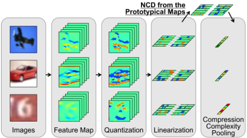
We observe that if we use qc l to quantize the prototypical map zcl of size H×W, only few quantization levels appear in the output map. This is because most values are collapsed to the average during the summarization of feature maps by Equation (9). Thus, we need to design an alternative quantizing function pcl for the prototypical map zcl . Let RTi be the rate of how many times the i-th quantization level γi appears among all the quantization levels in the training dataset. Then we quantize the prototypical map zcl so that the appearance rate RPi of the i-th quantization level γi observed from the quantized prototypical map pcl (zcl ) becomes similar to that from the training set (i.e., RTi). In other words, the quantizing function pcl satisfies the following conditions:
The prototypical map is obtained for each feature map, so the definition of the CCP should be revised accordingly. For the c-th feature map of the l-th layer f cl , Equations (7) and (8) can be rewritten based on the prototypical maps Z := {zcl for any l and c}:
3.2 MALCOM: Mahalanobis Detector with CCP Confidence Score for OOD Image Detection
To put it all together, we obtain twofold pooling vectors r that encode the spatial information by concatenating two vectors obtained by GAP and CCP.
where ρ(x;Z) :=‖Ll=1 ρl(x). Based on the twofold pooling vectors, we define a final OOD score function κ based on the Mahalanobis distance in order to remove the correlation between feature maps.
| Model | CIFAR-10 | CIFAR-100 | SVHN |
| DenseNet | 95.24(0.12) | 76.99(0.33) | 96.83(0.12) |
|---|---|---|---|
| ResNet | 95.24(0.24) | 78.20(0.41) | 96.18(0.20) |
Feature Ensemble
Even though we focus on the constrained OOD detection for our main motivation (Sec 2.1), we additionally propose an extended version of MALCOM, called MALCOM++, for the special case that some OOD samples are available for its validation and a specific OOD distribution can be assumed at test time. To be specific, MALCOM++ adopts the feature ensemble, which defines the final confidence score by the weighted sum of the scores computed from multiple hidden layers, and it turns out to be effective where we can infer the test distribution from a validation set of OOD samples [Lee et al., 2018b]. It is worth noting that MALCOM++ summarizes the scores directly from multiple layers based on hyperparameters rather than utilizes concatenation.
4 Experiments
4.1 Experimental Settings
Models and Datasets. We choose two popular deep neural networks used for image classification: DenseNet [Huang et al., 2017] with 100 layers and growth rate k=12, and ResNet [He et al., 2016] with 34 layers. We train the networks with a softmax layer and cross entropy loss using three datasets: CIFAR-10, CIFAR-100 [Krizhevsky et al., 2009] and SVHN [Netzer et al., 2011]. 2 In addition to the three training datasets (i.e., ID), we use four additional image datasets as OOD samples in test distributions: TinyImageNet [Deng et al., 2009], LSUN [Yu et al., 2015], and iSUN [Xu et al., 2015]. To train the networks, SGD with initial learning rate 0.1 and Nesterov momentum 0.9 is used, and the weight decay is set to 0.0001, 0.0005, and the batch size is set to 64 and 128, respectively for DenseNet and ResNet. We repeat to train the models five times and report their average results for all experiments. The test accuracy for the classification is reported in Table 2.
CompetingMethods. We compare the performance of our method with that of the existing methods which detect OOD samples using pretrained softmax classifier: ODIN [Liang et al., 2018] and Mahalanobis detector [Lee et al., 2018b]. Both the methods utilize OOD samples to find the optimal hyperparameters. In this sense, they do not satisfy our first constraint describing that any test distributions should not be assumed. Nevertheless, we loosen the constraint and report the results to show relative performance compared to the state-of-the-art methods. We utilize the publicly available codes of ODIN and Mahalanobis provided by previous work. 3
2 Our experiments follow most of the experimental settings mainly used in previous work [Liang et al., 2018; Lee et al., 2018b].
| Method | Layer 1 | Layer · · · | Layer L | DenseNet | ResNet | |||||
|---|---|---|---|---|---|---|---|---|---|---|
| GAP | CCP | GAP | CCP | GAP | CCP | SVHN | TinyIm | SVHN | TinyIm | |
| - | ✓ | - | - | - | - | - | 28.32 | 62.94 | 62.73 | 88.16 |
| - | - | ✓ | - | - | - | - | 84.21 | 63.58 | 85.16 | 62.76 |
| - | ✓ | ✓ | - | - | - | - | 67.61 | 67.13 | 83.39 | 87.36 |
| MV | - | - | - | - | ✓ | - | 91.19 | 95.39 | 82.65 | 86.20 |
| - | - | - | - | - | - | ✓ | 88.81 | 87.51 | 80.94 | 88.64 |
| - | - | - | - | - | ✓ | ✓ | 92.37 | 95.46 | 82.50 | 88.58 |
| MA | ✓ | - | ✓ | - | ✓ | - | 90.72 | 96.85 | 90.38 | 97.75 |
| - | - | ✓ | - | ✓ | - | ✓ | 96.03 | 89.19 | 95.00 | 93.46 |
| MALCOM | ✓ | ✓ | ✓ | ✓ | ✓ | ✓ | 94.34 | 96.93 | 94.50 | 97.91 |
| Model | Index | OOD | Random sample | Prototypical maps |
|---|---|---|---|---|
| DenseNet | 0 | SVHN TinyIm | 93.21(0.32) 96.38(0.13) | 93.59(0.08) 96.33(0.03) |
| ResNet | 1 | SVHN | 94.35(0.37) | 94.51(0.11) |
| TinyIm | 96.88(0.11) | 96.92(0.01) | ||
| 0 | SVHN | 92.74(0.91) | 93.69(0.12) | |
| TinyIm SVHN | 97.35(0.05) 94.68(0.55) | 97.58(0.02) 95.33(0.03) | ||
| 1 | TinyIm | 98.14(0.06) | 98.31(0.01) |
EvaluationMetrics. We adopt the three performance metrics the same with the previous work [Lee et al., 2018b]: true negative rate (TNR) at 95% true positive rate (TPR), area under the receiver operating characteristic curve (AUROC), and detection accuracy.
Implementation Details
We employ the Lempel-Ziv-Welch (LZW) coding scheme [Welch, 1984] for the compression algorithm Z used to compute the NCD. The NCD only requires the lengths of compression results, and the LZW coding scheme has an advantage of computing the length of an input string in O(n); we further accelerate the computation by using GPU.
We quantize the feature maps by using the Lloyd-Max quantizer [Lloyd, 1982; Max, 1960], which effectively minimizes the information loss. We fix the number of levels to 4, known to perform well for images when it used with our compression scheme (i.e., LZW) [Pinho and Ferreira, 2011]. Specifically, we use Lloyd-Max quantizer to obtain the thresholds for quantization after gathering all values of each feature map of the training samples.
We adopt the Hilbert space-filling curve to linearize the 2D feature maps. Among several linearizations, including simple row-wise (or column-wise) strategies, linearizing images by Hilbert space-filling curve turns out to be effective when using NCD for images [Liang et al., 2008]. Note that each feature map of l-th hidden layer has the same size of Hl×Wl, so the linearizing function λl is defined for each layer. Our code is publicly available. 4
3 https://github.com/pokaxpoka/deep Mahalanobis detector
4.2 Results
Effectiveness of the CCP
We ablate the components of our method to investigate the effectiveness of GAP, CCP, and their combinations. For rigorous analyses, we evaluate a wide range of Mahalanobis distance-based detectors, including MV, MA, and MALCOM; they apply either GAP or CCP, or both of them to the feature maps obtained from a single or multiple hidden layers. Table 3 presents the results of the ablation study.
In Table 3, the detector using only CCP or using both GAP and CCP on all hidden layers performs the best in most cases. More concretely, we observe that CCP brings more significant improvements when CCP is applied to lower-level features, especially the case that only the first hidden layer is used. On the contrary, in the case of the high-level features in the last hidden layer, CCP shows moderate performances and does not seem to have superiority compared to GAP. In this sense, the CCP which takes advantage of spatial information becomes much helpful to accurately detect OOD samples, particularly for lower-level features encoding more spatial information of input images. In conclusion, CCP greatly contributes to performance improvement and becomes much effective where GAP cannot derive meaningful information from low-level features.
Effectiveness of the Prototypical Maps. To demonstrate the effectiveness of the proposed prototypical maps, we compare MALCOM that uses a randomly selected sample for CCP (from Equation (8)) with the one that adopts prototypical maps for CCP (from Equation (11)). In Table 4, the standard deviation of MALCOM with the prototypical maps is consistently smaller than the one with a random sample, which indicates that the robustness of our NCD is improved as we intended. Furthermore, MALCOM with the prototypical maps also shows slightly better performances than the other. This implies that the prototypical maps help NCD to distinguish OOD samples by encoding the information of all training samples in itself.
Main Results
The main comparison results are summarized in Table 5. For each experiment, we leave out 1000 images from ID and OOD test sets and use them for the validation; thus, these 2000 images are not used for MALCOM which does not need to tune any hyperparameter.
In Table 5, our proposed methods (i.e., MALCOM and MALCOM++) outperform the state-of-the-art method in most cases. From the extensive experiments, we conclude that MALCOM is more effective to detect OOD samples compared to existing methods while it keeps satisfying the conditions for the constrained OOD detection. Furthermore, it can be easily extended to adopt the calibration technique, which further improves the performance by using OOD samples for its validation.
4 https://github.com/hunu12/MALCOM
| ID | OOD | TNR at 95% TPR | AUROC (ours) / MALCOM++ | Detection Accuracy (ours) |
|---|---|---|---|---|
| ODIN / MAHALANOBIS / MALCOM | ||||
| CIFAR-10 | CIFAR100 SVHN TinyIm(C) TinyIm(R) LSUN(C) LSUN(R) iSUN | 51.09(2.16) / 17.91(3.61) / 24.08(0.29) / 18.70(0.86) 81.26(6.05) / 92.28(2.01) / 95.40(0.64) / 96.58(0.40) 94.88(0.47) / 99.79(0.32) / 100.0(0.00) / 99.73(0.14) 87.59(2.09) / 93.61(2.29) / 94.71(0.36) / 95.50(0.53) 92.57(1.09) / 99.31(1.00) / 100.0(0.00) / 99.64(0.19) 94.53(0.87) / 96.21(1.43) / 95.32(0.74) / 96.78(0.60) 91.81(1.24) / 93.21(2.36) / 94.12(0.66) / 95.59(0.72) | 89.99(0.34) / 63.58(4.30) / 70.78(0.41) / 70.96(0.45) 94.46(2.11) / 98.23(0.64) / 98.94(0.11) / 99.19(0.06) 98.90(0.03) / 99.88(0.14) / 99.91(0.03) / 99.93(0.03) 97.69(0.33) / 98.29(1.00) / 98.88(0.09) / 99.06(0.13) 98.52(0.17) / 99.72(0.33) / 99.89(0.04) / 99.92(0.04) 98.85(0.15) / 98.91(0.45) / 98.91(0.14) / 99.23(0.15) 98.40(0.19) / 97.98(1.09) / 98.79(0.12) / 99.04(0.14) | 82.81(0.48) / 60.10(2.53) / 64.80(0.36) / 64.80(0.37) 90.01(2.39) / 93.96(0.89) / 95.25(0.33) / 95.94(0.19) 95.02(0.19) / 99.26(0.62) / 99.42(0.15) / 99.42(0.19) 92.34(0.75) / 94.38(1.14) / 94.91(0.20) / 95.33(0.33) 94.26(0.41) / 98.59(1.26) / 99.29(0.23) / 99.30(0.25) 94.91(0.43) / 95.78(0.74) / 95.23(0.33) / 96.07(0.39) 93.82(0.46) / 94.17(1.17) / 94.71(0.33) / 95.41(0.35) |
| DenseNet CIFAR-100 | CIFAR10 SVHN TinyIm(C) TinyIm(R) LSUN(C) LSUN(R) iSUN | 20.29(1.38) / 08.80(1.11) / 01.33(0.08) / 13.13(0.47) 66.16(8.55) / 76.33(6.73) / 66.15(2.78) / 87.46(0.91) 76.49(3.79) / 99.31(0.42) / 99.85(0.10) / 99.57(0.14) 53.88(4.71) / 80.37(2.47) / 82.67(2.29) / 87.12(1.48) 77.12(4.58) / 98.93(0.89) / 99.73(0.17) / 99.67(0.12) 60.77(5.61) / 85.74(1.46) / 82.60(3.14) / 90.46(1.70) 54.85(5.80) / 81.78(1.97) / 81.10(2.68) / 88.29(1.25) | 77.05(1.02) / 61.37(1.01) / 44.94(0.36) / 60.17(0.31) 92.87(2.50) / 91.61(3.50) / 94.34(0.39) / 96.76(0.23) 95.36(1.08) / 99.66(0.19) / 99.43(0.14) / 99.87(0.04) 89.16(2.65) / 93.64(1.70) / 96.93(0.36) / 97.21(0.33) 95.89(0.78) / 99.48(0.43) / 99.31(0.18) / 99.91(0.04) 92.06(1.94) / 95.82(0.74) / 96.94(0.43) / 97.61(0.38) 90.29(2.36) / 94.81(1.32) / 96.79(0.39) / 97.34(0.33) | 70.78(0.86) / 58.49(0.65) / 50.76(0.10) / 57.62(0.34) 85.77(3.11) / 87.02(3.48) / 88.16(0.51) / 91.52(0.36) 88.51(1.57) / 98.66(0.50) / 98.21(0.36) / 99.08(0.15) 81.32(2.72) / 88.40(1.53) / 91.10(0.59) / 91.65(0.58) 89.40(0.90) / 98.42(0.80) / 97.90(0.44) / 99.16(0.22) 84.51(2.50) / 90.85(0.85) / 91.66(0.73) / 92.87(0.74) 82.51(2.73) / 89.30(1.26) / 90.93(0.58) / 92.04(0.55) |
| SVHN | CIFAR10 CIFAR100 TinyIm(C) TinyIm(R) LSUN(C) LSUN(R) iSUN | 83.90(0.95) / 73.05(8.38) / 91.46(0.39) / 90.88(0.42) 80.90(0.84) / 84.27(2.07) / 92.75(0.41) / 91.56(0.51) 72.21(0.94) / 99.84(0.10) / 100.0(0.00) / 99.86(0.03) 81.02(0.97) / 93.28(3.78) / 98.65(0.24) / 97.04(0.23) 78.11(2.71) / 99.73(0.23) / 100.0(0.00) / 99.81(0.03) 77.80(2.60) / 97.02(1.36) / 99.25(0.19) / 97.14(0.29) 82.17(1.53) / 96.24(1.09) / 98.81(0.15) / 96.61(0.32) | 96.81(0.24) / 93.02(3.77) / 98.16(0.04) / 97.79(0.08) 96.08(0.33) / 96.83(0.48) / 98.34(0.07) / 97.99(0.08) 94.33(0.31) / 99.83(0.11) / 99.98(0.00) / 99.95(0.01) 96.28(0.15) / 97.93(1.33) / 99.46(0.02) / 99.21(0.04) 94.87(0.82) / 99.75(0.10) / 99.98(0.00) / 99.95(0.01) 95.52(0.54) / 98.99(0.34) / 99.51(0.03) / 99.20(0.05) 96.38(0.27) / 98.94(0.22) / 99.46(0.04) / 99.13(0.05) | 91.36(0.42) / 86.93(3.86) / 93.89(0.14) / 93.05(0.21) 90.42(0.53) / 91.42(0.69) / 94.28(0.13) / 93.39(0.23) 88.35(0.42) / 98.97(0.39) / 99.83(0.02) / 99.71(0.02) 90.61(0.16) / 94.25(1.88) / 97.19(0.15) / 96.33(0.19) 88.81(0.97) / 98.64(0.41) / 99.81(0.02) / 99.65(0.04) 89.59(0.66) / 96.20(0.77) / 97.63(0.18) / 96.56(0.30) 90.71(0.46) / 95.68(0.55) / 97.25(0.16) / 96.15(0.20) |
| CIFAR-10 | CIFAR100 SVHN TinyIm(C) TinyIm(R) LSUN(C) LSUN(R) iSUN | 47.44(1.42) / 47.64(1.16) / 47.57(1.26) / 58.96(0.92) 72.50(6.68) / 91.65(3.43) / 66.15(6.81) / 96.13(0.90) 71.68(3.18) / 99.93(0.15) / 89.92(2.60) / 99.92(0.03) 70.39(1.23) / 97.53(0.51) / 77.30(2.56) / 98.10(0.59) 77.46(2.59) / 99.89(0.19) / 89.15(2.77) / 99.87(0.05) 81.94(1.74) / 98.83(0.38) / 81.36(2.51) / 99.04(0.17) 77.89(1.76) / 97.64(0.47) / 80.11(2.71) / 98.25(0.32) | 83.83(1.33) / 89.27(0.37) / 89.81(0.25) / 89.62(0.18) 93.66(2.22) / 98.28(0.49) / 95.44(0.65) / 99.14(0.17) 91.67(1.33) / 99.90(0.15) / 98.30(0.28) / 99.97(0.01) 91.88(0.54) / 99.43(0.09) / 96.71(0.25) / 99.56(0.08) 94.32(1.21) / 99.85(0.18) / 98.26(0.33) / 99.96(0.01) 95.55(0.45) / 99.64(0.11) / 97.26(0.21) / 99.70(0.06) 94.26(0.50) / 99.47(0.08) / 97.01(0.27) / 99.59(0.05) | 78.44(1.21) / 82.19(0.65) / 83.16(0.35) / 82.98(0.24) 87.56(2.87) / 93.89(1.26) / 90.82(0.51) / 95.74(0.52) 86.79(1.11) / 99.43(0.16) / 94.59(0.34) / 99.72(0.07) 85.82(0.76) / 96.55(0.37) / 91.48(0.34) / 96.92(0.40) 89.17(1.04) / 98.97(0.27) / 94.27(0.38) / 99.63(0.12) 90.01(0.58) / 97.58(0.28) / 92.55(0.37) / 97.65(0.23) 88.40(0.67) / 96.66(0.27) / 92.05(0.38) / 96.94(0.25) |
| ResNet CIFAR-100 | CIFAR10 SVHN TinyIm(C) TinyIm(R) LSUN(C) LSUN(R) iSUN | 20.93(1.00) / 18.07(0.73) / 10.39(0.89) / 26.34(1.80) 79.34(5.16) / 89.65(2.84) / 71.93(3.38) / 91.08(1.73) 48.22(3.18) / 99.99(0.01) / 99.85(0.18) / 99.92(0.03) 64.48(5.98) / 91.76(0.88) / 89.41(1.61) / 92.88(0.79) 49.51(1.58) / 99.97(0.04) / 99.74(0.36) / 99.92(0.04) 64.95(8.58) / 95.31(0.76) / 90.19(3.02) / 94.76(0.75) 63.03(6.52) / 91.98(0.74) / 86.81(2.79) / 92.36(0.91) | 79.38(0.22) / 73.85(2.00) / 72.41(0.72) / 76.99(0.55) 96.01(0.90) / 97.85(0.52) / 94.50(0.62) / 97.84(0.46) 88.78(0.68) / 99.97(0.02) / 99.90(0.08) / 99.96(0.03) 93.06(1.19) / 98.28(0.18) / 97.91(0.28) / 98.54(0.19) 86.79(0.53) / 99.95(0.02) / 99.86(0.12) / 99.97(0.02) 93.39(1.89) / 98.81(0.13) / 97.98(0.54) / 98.71(0.16) 92.76(1.39) / 98.27(0.12) / 97.24(0.50) / 98.24(0.20) | 72.90(0.22) / 68.73(1.84) / 68.62(0.68) / 71.56(0.51) 90.33(1.03) / 93.17(0.86) / 87.35(0.98) / 93.20(0.74) 80.92(0.71) / 99.61(0.17) / 99.12(0.60) / 99.69(0.05) 85.77(1.47) / 93.56(0.38) / 92.50(0.72) / 94.10(0.35) 79.01(0.62) / 99.34(0.31) / 98.82(0.81) / 99.67(0.09) 86.09(2.17) / 95.22(0.38) / 92.92(1.25) / 94.92(0.40) 85.33(1.61) / 93.76(0.21) / 91.45(1.09) / 93.81(0.41) |
| SVHN | CIFAR10 CIFAR100 TinyIm(C) TinyIm(R) LSUN(C) LSUN(R) iSUN | 78.29(3.13) / 93.94(1.07) / 87.53(1.02) / 95.53(0.56) 76.78(3.15) / 94.05(1.17) / 87.88(0.94) / 95.65(0.66) 94.08(1.52) / 99.96(0.05) / 100.0(0.00) / 99.97(0.04) 78.68(3.32) / 98.71(0.35) / 95.18(0.45) / 98.53(0.42) 86.24(2.67) / 99.86(0.14) / 100.0(0.00) / 99.97(0.04) 78.21(3.54) / 99.02(0.41) / 94.38(0.83) / 98.72(0.38) 77.99(4.35) / 98.93(0.51) / 94.32(0.70) / 98.55(0.39) | 94.14(2.24) / 98.59(0.18) / 97.82(0.14) / 98.90(0.16) 94.34(1.15) / 98.56(0.21) / 97.88(0.16) / 98.89(0.20) 98.32(0.65) / 99.94(0.07) / 99.98(0.03) / 99.97(0.04) 94.17(2.61) / 99.47(0.14) / 98.95(0.09) / 99.60(0.15) 96.05(2.32) / 99.84(0.14) / 99.97(0.04) / 99.98(0.03) 93.80(2.93) / 99.53(0.12) / 98.82(0.13) / 99.62(0.11) 93.80(3.18) / 99.50(0.13) / 98.79(0.12) / 99.61(0.12) | 88.77(1.66) / 94.94(0.32) / 93.49(0.23) / 95.54(0.36) 88.91(0.61) / 94.87(0.41) / 93.38(0.23) / 95.52(0.40) 94.60(0.74) / 99.64(0.34) / 99.79(0.30) / 99.92(0.11) 88.93(1.86) / 97.16(0.34) / 95.30(0.21) / 97.60(0.40) 91.13(1.31) / 99.50(0.48) / 99.68(0.43) / 99.91(0.12) 88.64(1.98) / 97.50(0.36) / 95.05(0.29) / 97.77(0.35) 88.70(2.36) / 97.34(0.46) / 94.97(0.27) / 97.63(0.39) |
5 RelatedWork
Most previous work on OOD detection with softmax classifiers introduced parameters which help to enhance the performance. ODIN [Liang et al., 2018] designed two calibration techniques (i.e., temperature scaling and input preprocessing) to boost its performance by manipulating softmax outputs. [Vyas et al., 2018] proposed an objective to detect OOD samples based on an ensemble of classifiers, which are trained by partitioned sets of samples.The state-of-the-art method [Lee et al., 2018b] focuses on the internal features of the CNNs, while it involves hyperparameters for input preprocessing and logistic regression that aggregates confidence scores from each hidden layer.
Another line of research closely related to ours is NCD applications in the image-specific tasks [Lan and Harvey, 2005; Guha and Ward, 2014]. Since most compression methods take two strings as the input, most work mainly focused on quantization and linearization of input images. For example, [Mortensen et al., 2009] studied the robustness of the NCD for different linearizations on shifted or rotated images, and [Liang et al., 2008] investigated the effects of different compression methods for the NCD on medical images. Among them, [Coltuc et al., 2018] pointed out that using the NCD directly on raw images is not effective enough to measure the similarity, so they aggregated NCDs based on several filters to improve its robustness. Our work differs in that MALCOM applies the NCD to feature maps from CNNs rather than raw images or simply smoothed images.
6 Conclusion
This paper proposes MALCOM, which accurately measures the confidence score for OOD detection without using any hyperparameters and without retraining the model. To address the limitation of the existing methods that cannot exploit the spatial information of feature maps, we introduce the CCP which computes the outputs based on the NCD between two feature maps. Our extensive evaluation over image datasets shows that CCP leverages the spatial information of the feature maps, especially when being applied to low-level features, and this brings the performance improvement compared to the existing GAP. In addition, by using both the pooling techniques simultaneously, MALCOM achieves the best performance among all competing methods.
Acknowledgments
This research was supported by the NRF grant funded by the MSIT: (No. 2016R1E1A1A01942642) and (No. 2017M3C4A7063570), the IITP grant funded by the MSIT: (No. 2018-0-00584) and (IITP-2019-2011-1-00783).
@inproceedings{ijcai2020p337,
  title     = {Convolutional Neural Networks with Compression Complexity Pooling for Out-of-Distribution Image Detection},
  author    = {Yu, Sehun and Lee, Dongha and Yu, Hwanjo},
  booktitle = {Proceedings of the Twenty-Ninth International Joint Conference on
               Artificial Intelligence, {IJCAI-20}},
  publisher = {International Joint Conferences on Artificial Intelligence Organization},
  editor    = {Christian Bessiere},
  pages     = {2435--2441},
  year      = {2020},
  month     = {7},
  note      = {Main track},
  doi       = {10.24963/ijcai.2020/337},
  url       = {https://doi.org/10.24963/ijcai.2020/337},
}
TY - CPAPER TI - Convolutional Neural Networks with Compression Complexity Pooling for Out-of-Distribution Image Detection AU - Yu, Sehun AU - Lee, Dongha AU - Yu, Hwanjo T2 - Proceedings of the Twenty-Ninth International Joint Conference on Artificial Intelligence, IJCAI-20 PB - International Joint Conferences on Artificial Intelligence Organization PY - 2020 SP - 2435 EP - 2441 DO - 10.24963/ijcai.2020/337 UR - https://doi.org/10.24963/ijcai.2020/337 ER -Copied
Machine-readable versions of this paper, for tools and AI agents:





