
Bidirectional Adversarial Training for Semi-Supervised Domain Adaptation
Proceedings of the Twenty-Ninth International Joint Conference on Artificial Intelligence. Main track. Pages 934-940.
https://doi.org/10.24963/ijcai.2020/130
Keywords
- Computer Vision: Recognition: Detection, Categorization, Indexing, Matching, Retrieval, Semantic Interpretation
- Machine Learning: Transfer, Adaptation, Multi-task Learning
Abstract
Semi-supervised domain adaptation (SSDA) is a novel branch of machine learning that scarce labeled target examples are available, compared with unsupervised domain adaptation. To make effective use of these additional data so as to bridge the domain gap, one possible way is to generate adversarial examples, which are images with additional perturbations, between the two domains and fill the domain gap. Adversarial training has been proven to be a powerful method for this purpose. However, the traditional adversarial training adds noises in arbitrary directions, which is inefficient to migrate between domains, or generate directional noises from the source to target domain and reverse. In this work, we devise a general bidirectional adversarial training method and employ gradient to guide adversarial examples across the domain gap, i.e., the Adaptive Adversarial Training (AAT) for source to target domain and Entropy-penalized Virtual Adversarial Training (E-VAT) for target to source domain. Particularly, we devise a Bidirectional Adversarial Training (BiAT) network to perform diverse adversarial trainings jointly. We evaluate the effectiveness of BiAT on three benchmark datasets and experimental results demonstrate the proposed method achieves the state-of-the-art.
- [Berthelot et al., 2019] David Berthelot, Nicholas Carlini, Ian Goodfellow, Nicolas Papernot, Avital Oliver, and Colin A Raffel. Mixmatch: A holistic approach to semi- supervised learning. In Advances in Neural Information Processing Systems, pages 5050-5060, 2019.
- [Carlini and Wagner, 2017] Nicholas Carlini and David Wagner. Towards evaluating the robustness of neural networks. In 2017 IEEE Symposium on Security and Privacy, pages 39-57. IEEE, 2017.
- [Ganin and Lempitsky, 2014] Yaroslav Ganin and Victor Lempitsky. Unsupervised domain adaptation by backprop- agation. arXiv preprint arXiv:1409.7495, 2014.
- [Goodfellow et al., 2014] Ian J Goodfellow, Jonathon Shlens, and Christian Szegedy. Explaining and harnessing adversarial examples. arXiv preprint arXiv:1412.6572, 2014.
- [Grandvalet and Bengio, 2005] Yves Grandvalet and Yoshua Bengio. Semi-supervised learning by entropy minimiza- tion. In Advances in Neural Information Processing Sys- tems, pages 529-536, 2005.
- [He et al., 2016] Kaiming He, Xiangyu Zhang, Shaoqing Ren, and Jian Sun. Deep residual learning for image recognition. In Proceedings of the IEEE Conference on Computer Vision and Pattern Recognition, pages 770-778, 2016.
- [Krizhevsky et al., 2012] Alex Krizhevsky, Ilya Sutskever, and Geoffrey E Hinton. Imagenet classification with deep convolutional neural networks. In Advances in Neural In- formation Processing Systems, pages 1097-1105, 2012.
- [Laine and Aila, 2016] Samuli Laine and Timo Aila. Tem- poral ensembling for semi-supervised learning. arXiv preprint arXiv:1610.02242, 2016.
- [Liu et al., 2019] Hong Liu, Mingsheng Long, Jianmin Wang, and Michael Jordan. Transferable adversarial train- ing: A general approach to adapting deep classifiers. In International Conference on Machine Learning, pages 4013-4022, 2019.
- [Long et al., 2015] Mingsheng Long, Yue Cao, Jianmin Wang, and Michael I Jordan. Learning transferable fea- tures with deep adaptation networks. arXiv preprint arXiv:1502.02791, 2015.
- [Long et al., 2017] Mingsheng Long, Han Zhu, Jianmin Wang, and Michael I Jordan. Deep transfer learning with joint adaptation networks. In International Conference on Machine Learning, pages 2208-2217, 2017.
- [Long et al., 2018] Mingsheng Long, Zhangjie Cao, Jianmin Wang, and Michael I Jordan. Conditional adversarial do- main adaptation. In Advances in Neural Information Pro- cessing Systems, pages 1640-1650, 2018.
- [Miyato et al., 2016] Takeru Miyato, Andrew M Dai, and Ian Goodfellow. Adversarial training methods for semi-supervised text classification. arXiv preprint arXiv:1605.07725, 2016.
- [Miyato et al., 2018] Takeru Miyato, Shin-ichi Maeda, Masanori Koyama, and Shin Ishii. Virtual adversarial training: a regularization method for supervised and semi-supervised learning. IEEE Transactions on Pattern Analysis and Machine Intelligence, 41(8):1979-1993, 2018.
- [Park et al., 2018] Sungrae Park, JunKeon Park, Su-Jin Shin, and Il-Chul Moon. Adversarial dropout for supervised and semi-supervised learning. In Thirty-Second AAAI Confer- ence on Artificial Intelligence, 2018.
- [Peng et al., 2019] Xingchao Peng, Qinxun Bai, Xide Xia, Zijun Huang, Kate Saenko, and Bo Wang. Moment match- ing for multi-source domain adaptation. In Proceedings of the IEEE International Conference on Computer Vision, pages 1406-1415, 2019.
- [Rasmus et al., 2015] Antti Rasmus, Mathias Berglund, Mikko Honkala, Harri Valpola, and Tapani Raiko. Semi- supervised learning with ladder networks. In Advances in Neural Information Processing Systems, pages 3546- 3554, 2015.
- [Saito et al., 2017] Kuniaki Saito, Yoshitaka Ushiku, Tat- suya Harada, and Kate Saenko. Adversarial dropout regu- larization. arXiv preprint arXiv:1711.01575, 2017.
- [Saito et al., 2018] Kuniaki Saito, Kohei Watanabe, Yoshi- taka Ushiku, and Tatsuya Harada. Maximum classifier discrepancy for unsupervised domain adaptation. In Pro- ceedings of the IEEE Conference on Computer Vision and Pattern Recognition, pages 3723-3732, 2018.
- [Saito et al., 2019] Kuniaki Saito, Donghyun Kim, Stan Sclaroff, Trevor Darrell, and Kate Saenko. Semi- supervised domain adaptation via minimax entropy. In Proceedings of the IEEE International Conference on Computer Vision, pages 8050-8058, 2019.
- [Szegedy et al., 2013] Christian Szegedy, Wojciech Zaremba, Ilya Sutskever, Joan Bruna, Dumitru Erhan, Ian Goodfellow, and Rob Fergus. Intriguing properties of neural networks. arXiv preprint arXiv:1312.6199, 2013.
- [Tarvainen and Valpola, 2017] Antti Tarvainen and Harri Valpola. Mean teachers are better role models: Weight- averaged consistency targets improve semi-supervised deep learning results. In Advances in Neural Information Processing Systems, pages 1195-1204, 2017.
References were extracted automatically from the PDF and may contain errors.
Full text extracted automatically from the PDF; figures, tables and equations may differ. The PDF is the version of record.
1 Introduction
When Semi-Supervised Learning (SSL) [Rasmus et al., 2015; Laine and Aila, 2016; Tarvainen and Valpola, 2017] meets Domain Adaptation (DA) [Ganin and Lempitsky, 2014; Long et al., 2015; Long et al., 2017], there recently highlights an appealing task of Semi-Supervised Domain Adaptation (SSDA) [Saito et al., 2019]. SSDA refers to the problem that we not only have plentiful labeled source domain data and unlabeled target domain data, but a small amount of labeled target domain data, typically one or three per class. SSDA methods usually use labeled examples (from both source and target domain) to jointly train a network and use unlabeled examples to regularize it. However, the importance of the labeled target data is downplayed. Although the labeled target data are still scarce, they may provide effective clues to explore the connection between the source and target domain and bridge the gap between them, such as generating perturbed auxiliary examples between two domains. As the triangle class in Fig. 1, the BiAT examples are generated from both the source domain → and the target domain , → , and fill the domain gap.
∗Equal contributions
†Corresponding author
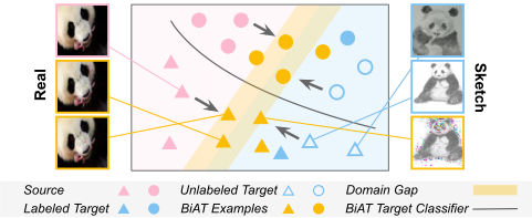
Corrupting training data with noises have been well-known to be helpful in stabilizing prediction [Park et al., 2018]. Recently, gradient-based perturbation generation methods, i.e., Adversarial Training (AT) [Goodfellow et al., 2014] as well as Virtual Adversarial Training (VAT) [Miyato et al., 2018], are proposed to generate adversarial examples, which are images with additional perturbations. Adversarial examples have been proven to be effective on supervised and semisupervised tasks [Miyato et al., 2016; Miyato et al., 2018]. The effectiveness owns to their ability of local smoothness around data points, and pushing decision boundary away from data points, which leads to an improvement of the model robustness for raw examples. However, it is not straightforward to use AT or VAT in SSDA. The noise direction of AT and VAT is arbitrary, which cannot make the adversarial examples cross the domain gap.
To solve the SSDA problem, an intuitive idea is to force AT and VAT to generate adversarial examples between the two domains and fill the domain gap. [Liu et al., 2019] introduced adversarial training at the feature layer to enhance the unsupervised domain adaptation. However, they use traditional AT on the source and target examples. The generated examples surround the original examples, which has only limited ability to fill the domain gap.
In order to guide the direction of generating adversarial examples from one domain towards another, we devise two opposing adversarial training methods which form a bidirectional strategy. We firstly propose Adaptive Adversarial Training (AAT), a novel adversarial training notion for specific SSDA scenarios that generates adaptive adversarial examples from the source to target domain. AAT treats a source example xs as a optimizable object, which is fed into a welltrained target domain classifier, then the target domain classifier will optimize xs along the direction of gradient descent and force xs to cross into the target domain. Moreover, we introduce Entropy-penalized Virtual Adversarial Training (EVAT) which improves VAT and generates adversarial examples from the target to source domain. Finally, we propose a uniform Bidirectional Adversarial Training (BiAT) network to perform AT, AAT, and E-VAT jointly. We evaluate BiAT on three benchmark datasets and conduct extensive ablation study. Experiments show the BiAT network advances all the state-of-the-arts.
Our contributions can be summarized into threefold. (1) We devise a novel Adaptive Adversarial Training for specific SSDA setting that generates adversarial examples from the source to target domain. (2) We introduce the Entropypenalized Virtual Adversarial Training to generate more accurate adversarial examples from the target to source domain. (3) We propose a uniform Bidirectional Adversarial Training network to integrate three adversarial training methods and demonstrate the effectiveness of them in SSDA scenarios.
2 RelatedWork
Semi-Supervised Domain Adaptation. SSDA was highlighted by [Saito et al., 2019] recently, which is a combination of semi-supervised learning (SSL) and domain adaptation (DA). The MME method they proposed maximize the entropy of unlabeled target data to optimize classifier, and minimize the entropy with respect to the feature extractor to cluster features. Recently, some effective arts of SSL have emerged. [Grandvalet and Bengio, 2005] considered entropy minimization as a regularizer to incorporate unlabeled data. [Laine and Aila, 2016] introduced ∏-model and temporalensembling, a consensus prediction of the unknown labels using an exponential moving average of outputs. [Berthelot et al., 2019] proposed MixMatch data-augment to generate lowentropy pseudo-labels. On the other hand, previous works have addressed the unsupervised DA problem which generalizes a learner across different domains, by either matching the marginal distributions or the conditional distributions [Long et al., 2018].
Adversarial Training. AT was proposed by [Szegedy et al., 2013] originally. They discovered that deep networks are particularly vulnerable to minor adversarial perturbations applied to the input. [Goodfellow et al., 2014] proposed the definition of adversarial examples and pointed out that adversarial training can restraint the impact of adversarial perturbations to some extent. Not just defense against adversarial attacks, adversarial training can also promise a variety of machine learning tasks. [Miyato et al., 2018] introduced virtual adversarial training in supervised and semi-supervised scenarios to promote local smoothness around data points.
3 Preliminaries
3.1 Adversarial Training
Adversarial Training is recognized as an effective method to improve the robustness of models [Szegedy et al., 2013; Goodfellow et al., 2014], which promotes the local smoothness and mitigates over-fitting by regularizing the network.
For labeled input pair (xl, yl) and unlabeled input xu, we denote the output distribution parameterized by Θ as p(y|x, Θ). The loss function of adversarial training in [Goodfellow et al., 2014] can be written as
D[·, ·] is a function that measures the divergence between two distributions. The q(yl) is the true distribution of label which is generally approximated by one-hot vector of yl.
When the norm is ℓ2, [Miyato et al., 2016] proposed to approximate the adversarial perturbation radv by
g is the gradient that can be efficiently computed by backpropagation, ϵ is the perturbation amplitude.
3.2 Virtual Adversarial Training
When facing unsupervised or semi-supervised learning tasks, [Miyato et al., 2018] proposed Virtual Adversarial Training which replaces the true label q(yl) in Eq.(1) with its current approximation p(y|xl, ˆΘ). Let x⋆ represents either xl or xu. The objective function is given by
Then Lvadv(x∗, Θ) can be considered as a regularization term over all input examples.
4 Bidirectional Adversarial Training
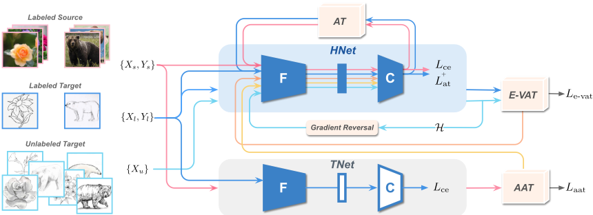
In this section, we propose a novel Bidirectional Adversarial Training (BiAT) method for SSDA task, illustrated in Fig. 2. We devise two opposing adversarial training which form a bidirectional strategy of adversarial example generation. AAT produces adversarial examples from the source to target domain in Section 4.2. E-VAT generates examples from the target to source domain, elaborated in Section 4.3. In addition, we combine the AT, AAT, E-VAT, and the minimax entropy method [Saito et al., 2019] to jointly construct an end-to-end network in Section 4.4.
<
l
a
t
e
x
i
s
h
1
_
b
6
4
=
"
r
G
/
v
T
w
R
q
7
A
k
Y
0
Q
E
>
C
B
H
c
V
D
L
S
N
F
J
3
U
2
M
u
o
g
W
9
p
+
y
O
Z
z
K
5
j
n
d
8
X
f
I
m
P
<
l
a
t
e
x
i
s
h
1
_
b
6
4
=
"
I
8
v
N
u
0
7
H
z
q
A
c
B
+
r
>
C
V
D
L
S
F
J
3
U
2
M
o
g
Q
k
W
9
p
y
Y
O
Z
G
E
K
5
j
n
d
X
f
/
m
w
R
P
T
<
l
a
t
e
x
i
s
h
1
_
b
6
4
=
"
u
O
I
3
Z
f
L
N
5
w
p
X
R
H
0
C
U
Y
D
>
A
B
/
c
V
S
F
J
2
v
+
G
y
q
K
o
M
7
E
T
g
k
z
9
j
n
W
d
P
r
m
8
Q
<
l
a
t
e
x
i
s
h
1
_
b
6
4
=
"
U
y
5
k
v
d
C
O
/
m
Y
j
G
r
f
M
>
A
B
+
X
c
V
N
S
8
E
3
q
o
9
L
0
P
R
w
F
H
p
2
D
T
W
z
Z
u
7
I
J
K
g
n
Q
<
l
a
t
e
x
i
s
h
1
_
b
6
4
=
"
G
N
v
3
P
/
8
O
M
A
K
E
L
k
n
y
F
I
>
B
c
V
S
J
U
r
q
9
0
R
w
W
p
2
Y
T
d
C
f
Z
X
j
o
7
Q
D
z
m
5
u
+
H
g
<
l
a
t
e
x
i
s
h
1
_
b
6
4
=
"
U
y
5
k
v
d
C
O
/
m
Y
j
G
r
f
M
>
A
B
+
X
c
V
N
S
8
E
3
q
o
9
L
0
P
R
w
F
H
p
2
D
T
W
z
Z
u
7
I
J
K
g
n
Q
<
l
a
t
e
x
i
s
h
1
_
b
6
4
=
"
E
I
q
N
S
P
d
v
u
L
n
+
D
Z
>
A
B
8
c
V
F
2
p
r
f
o
g
Q
K
9
J
0
m
Y
G
W
T
O
y
7
X
k
H
/
5
3
U
j
C
R
z
M
w
<
l
a
t
e
x
i
s
h
1
_
b
6
4
=
"
W
O
c
H
J
r
S
L
3
n
8
0
z
C
G
E
>
A
B
V
N
U
q
/
9
Z
o
g
X
j
y
2
Y
D
+
R
5
u
w
F
K
k
v
p
P
m
7
T
Q
d
f
I
M
<
l
a
t
e
x
i
s
h
1
_
b
6
4
=
"
W
O
c
H
J
r
S
L
3
n
8
0
z
C
G
E
>
A
B
V
N
U
q
/
9
Z
o
g
X
j
y
2
Y
D
+
R
5
u
w
F
K
k
v
p
P
m
7
T
Q
d
f
I
M
<
l
a
t
e
x
i
s
h
1
_
b
6
4
=
"
W
O
c
H
J
r
S
L
3
n
8
0
z
C
G
E
>
A
B
V
N
U
q
/
9
Z
o
g
X
j
y
2
Y
D
+
R
5
u
w
F
K
k
v
p
P
m
7
T
Q
d
f
I
M
<
l
a
t
e
x
i
s
h
1
_
b
6
4
=
"
m
7
Z
g
Y
O
8
W
X
q
M
3
P
0
F
d
2
u
Q
>
A
B
9
c
V
D
L
S
N
E
J
z
G
r
H
C
w
k
j
T
n
I
y
v
5
p
U
R
/
o
+
f
K
<
l
a
t
e
x
i
s
h
1
_
b
6
4
=
"
L
M
m
Z
9
g
N
T
8
0
q
U
Q
n
I
>
A
B
3
c
V
S
E
r
/
G
P
R
w
F
W
K
p
2
Y
d
C
f
X
j
o
7
D
z
v
5
y
u
+
k
O
J
H
4.1 Semi-Supervised Domain Adaptation
Under the SSDA setting, the data comes from two different domains, the source domain S and the target domain T . Data from the source domain S = {Xs, Ys} are labeled, and each data point xs ∈ Xs has an associated label ys ∈ Ys. A small number of target domain data are labeled (one or three per class), formalized as Tl = {Xl, Yl} that data point xl ∈ Xl has an associated label yl ∈ Yl. The rest is unlabeled target domain data Tu = {Xu}. Our goal is to find a model that performs well on unlabeled target domain test data.
Similar to the previous domain adaptation models [Ganin and Lempitsky, 2014; Saito et al., 2018], our backbone network consists of two modules, the feature extractor F and the classifier C. We can employ commonly used deep convolutional neural networks as feature extractors, such as AlexNet [Krizhevsky et al., 2012] and ResNet [He et al., 2016]. We denote the network outputs as h = C(F (x)), ∈ Rc .
Previously, [Saito et al., 2019] has shown that performing ℓ2 normalization on the outputs of F achieves good performance. We further conduct weight normalization on the classifier. We write the weight matrix WC ∈ Rd×c as [w1,w2, ...,wc], where each class corresponds to a ddimensional weight vector. Then C takes normalized features as input and calculate the cosine similarity scores to weight vectors as h = 1 T F (x)TWC ‖F(x)‖‖WC‖ , where T is the temperature parameter. Consequently, the outputs is the prediction scores of corresponding classes. Then the weight vectors of WC can be interpreted as prototypes of classes, which may be effective due to reducing intra-class variations.
4.2 Adaptive Adversarial Training
Here, we propose Adaptive Adversarial Training (AAT), a novel adversarial training notion for SSDA task that can generate adaptive adversarial examples to fill the domain gap from the source to target domain (S → T ). Unlike traditional adversarial training, which adds arbitrary perturbation to examples in a single domain, our AAT adds perturbation in a direction and can indicate the direction of domain adaptation.
In AAT, we can access to plentiful labeled source data, and other small amount of labeled target data. Suppose we can find a clear direction to guide the source examples towards the target domain, then we use these adversarial examples to train the network may effectively improve the performance.
Main Idea. The goal of AAT is to generate directional perturbation on a source example, and more importantly, the direction should point to the target examples of the same class. Following the idea of adversarial training, we employ the gradients to do this work. The novel idea is to treat a source example xs as an optimizable object, which is fed into a frozen well-trained target domain network TNet. Since the TNet can only recognize target data, then TNet will optimize xs along the direction of gradient descent and force xs to cross into the target domain. Note that, this optimization process only occurs in the example space and the optimized examples are regarded as adaptive adversarial examples. The AAT is inspired by targeted adversarial attack which aims to generate adversarial examples targeting a specific class from a given image and regards the direction of gradient descent as the direction of noises [Carlini and Wagner, 2017].
We first train a capable TNet as ΘT using all the labeled target data Tl. Then we froze ΘT and feed the source data S = {Xs, Ys} into the network and generate adaptive adversarial examples by the direction of gradient descent. With the ℓ2 norm, the adversarial perturbation can be approximated by
The only difference from traditional AT is that the network for gradients becomes ΘT . The loss function of AAT is
where Θ denotes the task-specific network.
4.3 Entropy-penalized Virtual Adversarial Training
In contrast to AAT, we introduce Entropy-penalized Virtual Adversarial Training (E-VAT) to generate adversarial examples from the target to source domain (T → S), following the philosophy of VAT. As mentioned in Section 3.2, VAT uses approximation method to generate perturbations on unlabeled examples and ensures consistency of network predictions. This makes the adversarial examples towards the source domain to some extent. However, limited by the lack of clear labels, traditional VAT is insufficient in SSDA task.
We make three improvements to the traditional VAT: (1) We use multi-step iteration to obtain more accurate adversarial perturbations; (2) In order to obtain clear supervision, we use hard pseudo-labels, i.e. one-hot labels, instead of ambiguous approximate predictions p(y|x∗ , ˆΘ) in VAT; (3) We introduce two entropy-based consistency penalization to obtain more consistent pseudo-labels and prioritize the highconfidence examples, respectively.
We first start E-VAT from a small random noise, and then follow the direction of gradient ascent to iteratively obtain multiple small perturbations. Although the noise direction of E-VAT is arbitrary, it is responsible for smoothing the local space and filling the domain gap to some extent. Each iteration of E-VAT corresponds to a classifier prediction. These outputs form a prediction matrix H = [h1, h2, ..., hN] ∈ RN×d , where hn denotes the prediction of n-th iteration and N is the number of iterations.
Row-wise and column-wise entropy penalty. For unlabeled examples, the pseudo-labels of N iterations may be inconsistent, especially in the early stage of training, which will confuse the pseudo-labels, e.g. the one-hot labels of h1 and hN may be different. For a vector, entropy is maximized if the distribution is uniform. We propose to penalize H that we want low row-wise entropy for clear predictions with high confidence, and high column-wise entropy to encourage consistent predictions in N iterations, so as to obtain an explicit pseudo-label. We quantify the row-wise and column-wise entropy penalty as weight scores.
Example-specific entropy penalty. Owing to the VAT sometimes gives a multi-peak prediction. This phenomenon suggests that such examples near the prototypes of two or more classes, and the wrong pseudo-label will mislead the model. Therefore, we introduce the example-specific entropy penalty to suppress these examples corresponding to small entropy He = - ∑d p(h′ ) log p(h′ ) and the examplespecific weight scores denote as We = e-He .
4.4 Bidirectional Adversarial Training Network
As shown in Fig. 2, we design two parallel networks, hybrid domain network HNet and target domain network TNet. We first use the labeled data S ∪ Tl to jointly train the HNet and use only the labeled target data Tl to train the TNet, used to assist AAT according to Section 4.2. We denote the parameters of feature extractor F as ΘF , classifier C as ΘC. To avoid overfitting, we freeze the F of TNet and share the parameters with HNet. Then we have ΘT = {ΘF ,ΘTC } and ΘH = {ΘF , ΘHC }.
Algorithm 1 Bidirectional Adversarial Training (BiAT)
Input: Source data S; Target labeled data Tl; Target unlabeled data Tu; Parameters of HNet ΘH; Parameters of TNet ΘT ; Batch size N.
- 1: while not converged do
- 2: Sample a mini-batch of N examples from S and Tl separately, 2N examples from Tu
- 3: // optimize HNet with cross entropy, AT, AAT, and EVAT
- 4: ΘH ←Lce(Xs,Xl, Ys, Yl,ΘH)
- 5: ΘH ←Lat(Xs,Xl, Ys, Yl,ΘH)
- 6: ΘH ←Laat(Xs, Ys,ΘT ,ΘH)
- 7: ΘH ←Le-vat(Xl,Xu,ΘH)
- 8: // optimize TNet with cross entropy
- 9: ΘT ←Lce(Xl, Yl,ΘT )
- 10: // optimize HNet with minimax entropy
- 11: ΘH ←Lmme(Xu,ΘH)
- 12: end while
- 13: return solution
In order to generate adversarial examples between the source and target domain, we propose the Bidirectional Adversarial Training mechanism to perform AT, AAT, and EVAT on the HNet jointly. In addition, we use the minimax entropy as an regular term because of the good performance [Saito et al., 2019]. We devise a three-stage training strategy in a mini-batch, shown in Algorithm 1. At first, we optimize the HNet with the cross entropy, AT, AAT, and E-VAT. Secondly, we optimize the classifier of TNet. Thirdly, we apply the minimax entropy regularization to HNet.
Task-specific objective. We define the task-specific objective function regarding the labeled data {X, Y } = {Xs ∪ Xl, Ys ∪ Yl}. As for classification task, the training objective of HNet is typical defined as cross entropy loss
AT objective. According to the Section 3.1, we use the labeled data S ∪ Tl to conduct traditional AT, the training objective can be written as Lat(X, Y, ΘH).
AAT objective. We use the labeled source data for AAT to generate adaptive adversarial examples from the source to target domain. The training objective is Laat(Xs, Ys, ΘT , ΘH).
E-VAT objective. We employ the E-VAT with unlabeled data on HNet to generate adversarial examples from the target to source domain. The VAT objective can be written as Le-vat(Xl , Xu, ΘH ).
Minimax Entropy objective. We apply the previous minimax entropy objective on classifier to maximize the entropy H of unlabeled target data, and minimize the entropy with respect to the feature extractor to cluster features [Saito et al., 2019], which form an adversarial minimax process. We use the gradient reversal layer to simplify the training process.
| Net | Methods | R → C | R → P | P → C | C → S | S → P | R → S | P → R | Mean | ||||||||
|---|---|---|---|---|---|---|---|---|---|---|---|---|---|---|---|---|---|
| 1-shot | 3-shot | 1-shot | 3-shot | 1-shot | 3-shot | 1-shot | 3-shot | 1-shot | 3-shot | 1-shot | 3-shot | 1-shot | 3-shot | 1-shot | 3-shot | ||
| S+T | 43.3 | 47.1 | 42.4 | 45.0 | 40.1 | 44.9 | 33.6 | 36.4 | 35.7 | 38.4 | 29.1 | 33.3 | 55.8 | 58.7 | 40.0 | 43.4 | |
| DANN | 43.3 | 46.1 | 41.6 | 43.8 | 39.1 | 41.0 | 35.9 | 36.5 | 36.9 | 38.9 | 32.5 | 33.4 | 53.6 | 57.3 | 40.4 | 42.4 | |
| AlexNet ADR | 43.1 | 46.2 | 41.4 | 44.4 | 39.3 | 43.6 | 32.8 | 36.4 | 33.1 | 38.9 | 29.1 | 32.4 | 55.9 | 57.3 | 39.2 | 42.7 | |
| CDAN | 46.3 | 46.8 | 45.7 | 45.0 | 38.3 | 42.3 | 27.5 | 29.5 | 30.2 | 33.7 | 28.8 | 31.3 | 56.7 | 58.7 | 39.1 | 41.0 | |
| ENT | 37.0 | 45.5 | 35.6 | 42.6 | 26.8 | 40.4 | 18.9 | 31.1 | 15.1 | 29.6 | 18.0 | 29.6 | 52.2 | 60.0 | 29.1 | 39.8 | |
| MME | 48.9 | 55.6 | 48.0 | 49.0 | 46.7 | 51.7 | 36.3 | 39.4 | 39.4 | 43.0 | 33.3 | 37.9 | 56.8 | 60.7 | 44.2 | 48.2 | |
| BiAT | 54.2 | 58.6 | 49.2 | 50.6 | 44.0 | 52.0 | 37.7 | 41.9 | 39.6 | 42.1 | 37.2 | 42.0 | 56.9 | 58.8 | 45.5 | 49.4 | |
| S+T | 55.6 | 60.0 | 60.6 | 62.2 | 56.8 | 59.4 | 50.8 | 55.0 | 56.0 | 59.5 | 46.3 | 50.1 | 71.8 | 73.9 | 56.9 | 60.0 | |
| DANN | 58.2 | 59.8 | 61.4 | 62.8 | 56.3 | 59.6 | 52.8 | 55.4 | 57.4 | 59.9 | 52.2 | 54.9 | 70.3 | 72.2 | 58.4 | 60.7 | |
| ResNet ADR | 57.1 | 60.7 | 61.3 | 61.9 | 57.0 | 60.7 | 51.0 | 54.4 | 56.0 | 59.9 | 49.0 | 51.1 | 72.0 | 74.2 | 57.6 | 60.4 | |
| CDAN | 65.0 | 69.0 | 64.9 | 67.3 | 63.7 | 68.4 | 53.1 | 57.8 | 63.4 | 65.3 | 54.5 | 59.0 | 73.2 | 78.5 | 62.5 | 66.5 | |
| ENT | 65.2 | 71.0 | 65.9 | 69.2 | 65.4 | 71.1 | 54.6 | 60.0 | 59.7 | 62.1 | 52.1 | 61.1 | 75.0 | 78.6 | 62.6 | 67.6 | |
| MME | 70.0 | 72.2 | 67.7 | 69.7 | 69.0 | 71.7 | 56.3 | 61.8 | 64.8 | 66.8 | 61.0 | 61.9 | 76.1 | 78.5 | 66.4 | 68.9 | |
| BiAT | 73.0 | 74.9 | 68.0 | 68.8 | 71.6 | 74.6 | 57.9 | 61.5 | 63.9 | 67.5 | 58.5 | 62.1 | 77.0 | 78.6 | 67.1 | 69.7 | |
| Methods | Office (W→A) | Office (D→A) | Office-Home | |||
|---|---|---|---|---|---|---|
| 1-shot | 3-shot | 1-shot | 3-shot | 1-shot | 3-shot | |
| S+T | 50.4 | 61.2 | 50.0 | 62.4 | 44.1 | 50.0 |
| DANN | 57.0 | 64.4 | 54.5 | 65.2 | 45.1 | 50.3 |
| ADR | 50.2 | 61.2 | 50.9 | 61.4 | 44.5 | 49.5 |
| CDAN | 50.4 | 60.3 | 48.5 | 61.4 | 41.2 | 46.2 |
| ENT | 50.7 | 64.0 | 50.0 | 66.2 | 38.8 | 50.9 |
| MME | 57.2 | 67.3 | 55.8 | 67.8 | 49.2 | 55.2 |
| BiAT | 57.9 | 68.2 | 54.6 | 68.5 | 49.6 | 56.4 |
Overall objectives. The overall training objective for training HNet can be written as
where λ1, λ2, λ3, λ4 are hyper-parameters. Lmme is a simplified form of LFmme and LCmme .
In addition, the training objective of TNet is
The whole training process is shown in Algorithm 1.
5 Experiments
5.1 Experimental Setup
Datasets. We address the SSDA problem and validate the benefits of BiAT on three datasets. DomainNet is a recent benchmark dataset for large-scale domain adaptation that has 6 domains and 345 classes [Peng et al., 2019]. Following the setup of [Saito et al., 2019], we pick 4 domains (Real, Clipart, Painting, Sketch) and 126 classes to construct 7 scenarios, shown in the first row of Table 1. Office contains 3 domains with 31 classes and we eliminate the domains with less examples and construct 2 scenarios, Webcam to Amazon (W→A) and DSLR to Amazon (D→A). Office-Home contains 4 domains (Real, Clipart, Art, Product) with 65 classes. For each dataset, we use the randomly selected one or three labeled examples per class as the labeled target examples (1shot and 3-shot) by [Saito et al., 2019]. Other three labeled target examples are used as validation set and the remaining are used as unlabeled target data.
| Methods | R→C | R→S | ||
|---|---|---|---|---|
| 1-shot | 3-shot | 1-shot | 3-shot | |
| Baseline (S+T) | 43.3 | 47.1 | 29.1 | 33.3 |
| Baseline w/ AT | 48.7 | 52.6 | 32.5 | 39.0 |
| Baseline w/ AAT | 46.6 | 49.6 | 31.6 | 36.6 |
| Baseline w/ E-VAT | 46.5 | 49.2 | 30.9 | 35.7 |
| BiAT w/o AT | 50.8 | 55.4 | 33.0 | 39.6 |
| BiAT w/o AAT | 49.8 | 54.7 | 31.3 | 37.7 |
| BiAT w/o E-VAT | 50.6 | 53.4 | 34.6 | 40.5 |
| BiAT w/o MME | 46.0 | 53.5 | 29.0 | 35.1 |
| BiAT | 54.2 | 58.6 | 37.2 | 42.0 |
Implementation details. For fair comparisons with other methods, we follow previous work and take the shallow network AlexNet [Krizhevsky et al., 2012] and deep network ResNet34 [He et al., 2016] as the backbones. We employ a shared pre-trained network as feature extractor and randomly initialized classifiers for both HNet and TNet. We set λ1 in Eq. (11) as 1, λ2 as 2. To avoid misjudgments of Le-vat in early training, we use cosine warm-up on λ3. Lmme is sensitive to datasets, even sub-domains of a same dataset, and we choose λ4 ∈ [0.1, 2.5] for different scenarios. We adopt SGD as an optimizer with initial learning rate 0.01. In order to make a fair comparison, other setup we choose the same as [Saito et al., 2019].
5.2 The Analysis of Experimental Results
We compare our BiAT network against several baselines. "S+T" is the model trained with labeled data (both source and target) and without unlabeled data. DANN [Ganin and Lempitsky, 2014], ADR [Saito et al., 2017], and CDAN [Long et al., 2018] are advanced unsupervised domain adaptation methods. ENT is the model jointly trained by source and target labeled data, and unlabeled target data are employed for standard entropy minimization. MME [Saito et al., 2019] is the SSDA method with only minimax entropy loss.
DomainNet. In Table 1, we show the detailed comparison on DomainNet dataset. Our BiAT method outperforms the most recent MME method on average by 1.3% (1-shot) and 1.2% (3-shot) with AlexNet, 0.7% (1-shot) and 0.8% (3-shot)
with ResNet. The result demonstrates that our BiAT method is effective in both shallow and deep networks. In some highquality scenarios with Real images as source, taking AlexNet as an example, we achieve outstanding performance boost at 5.3% and 3.0% on R→C, 3.9% and 4.1% on R→S with 1shot and 3-shot, separately.
Office and Office-Home. In Table 2, we show the experimental results on Office and Office-Home dataset. In the two scenarios of Office, BiAT demonstrates comparable performance, which is only behind the MME on D→A (1-shot). That may be due to the DSLR set is small with only hundreds of images and less data are inefficient to fill the domain gap. For the Office-Home dataset, BiAT achieves a best overall accuracy at 49.6% (1-shot) and 56.4% (3-shot), outperforming 0.4% and 1.2% than the prior state-of-the-art.
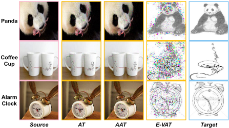
In Fig. 3, we visualize the adversarial examples from BiAT on the DomainNet dataset. The middle three columns show the generated examples with additional perturbations from AT, AAT, and E-VAT, respectively.
5.3 Ablation Study
In order to exploit different model variants and analyze the effectiveness, we conduct ablation study in two scenarios on DomainNet, R→C and R→S, shown in Table 3.
We regard the "S+T" model as the baseline of BiAT without adversarial training methods. As can be seen in the first part of Table 3, AT apparently boosts the accuracy by around 4% from baseline on all the scenarios. AAT can promote the baseline by around 3% accuracy. Similarly, E-VAT achieves around 3% accuracy improvements. These two results not only show the validity of the BiAT methods, but also indicate the two generation directions are almost equally important.
As shown in the second part of Table 3, it causes a decline in performance without any adversarial training methods. This proves that all the adversarial training components are necessary. Note that the MME is also used as a term for stable training, and it is sensitive to hyper-parameters. Simply removing the MME may lead to poor performance, such as the R→S (1-shot) case. When all methods are combined, the scores of the BiAT demonstrate the effectiveness of BiAT.
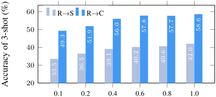
Varying number of bidirectional adversarial examples. We take the number of bidirectional adversarial examples as a variable and analyse the effort of example size. As shown in Fig. 4, the horizontal axis represents the ratio of adversarial examples. The ratio increases from left to right, and "1.0" indicates all the adversarial examples are used, i.e. 2N AT examples, N AAT examples, and 2N E-VAT examples in a mini-batch, where N is the batch size. Obviously, the increase of example size significantly improves the accuracy of the model. This result is quite reasonable, because more adversarial examples can better smooth the data points, and fill the gaps between domains, thus learning a capable classifier.
5.4 Discussion of BiAT
In general, our BiAT method is validated to be valid on all the three datasets and has around 1% accuracy improvement on average. Because BiAT is essentially a data enhancement method and does not innovate the image recognition backbone, it is reasonable that BiAT cannot greatly improve the classification performance. Even so, BiAT still performs well in many cases (around 5% accuracy improvements). In addition, as a general adversarial training paradigm, BiAT can universally boost models, which can be regarded as a plugin method for SSDA or other domain adaptation tasks. As long as there is an input example and a network that can give a clear gradient direction, AAT can guide the perturbation along the desired direction and obtain the corresponding adversarial examples. For unsupervised data, E-VAT is also universal. We argue that the BiAT method can act as a general technique for SSDA or other domain adaptation problem.
6 Conclusion
In this paper, we devise a general bidirectional adversarial training method and employ gradient to guide adversarial examples across domain gap and fill the gap. We propose two effective components, AAT and E-VAT. AAT generates adaptive adversarial examples from the source to target domain, while E-VAT does the opposite. We evaluate our method on three benchmark datasets and conduct extensive ablation study to the effectiveness of the BiAT. Experiments show the network achieves the state-of-the-art.
Acknowledgments
This work is supported by the NSFC (under Grant 61876130, 61932009). Thanks to Huawei Noah's Ark Lab NetMIND Research Team for funding this research.
@inproceedings{ijcai2020p130,
  title     = {Bidirectional Adversarial Training for Semi-Supervised Domain Adaptation},
  author    = {Jiang, Pin and Wu, Aming and Han, Yahong and Shao, Yunfeng and Qi, Meiyu and Li, Bingshuai},
  booktitle = {Proceedings of the Twenty-Ninth International Joint Conference on
               Artificial Intelligence, {IJCAI-20}},
  publisher = {International Joint Conferences on Artificial Intelligence Organization},
  editor    = {Christian Bessiere},
  pages     = {934--940},
  year      = {2020},
  month     = {7},
  note      = {Main track},
  doi       = {10.24963/ijcai.2020/130},
  url       = {https://doi.org/10.24963/ijcai.2020/130},
}
TY - CPAPER TI - Bidirectional Adversarial Training for Semi-Supervised Domain Adaptation AU - Jiang, Pin AU - Wu, Aming AU - Han, Yahong AU - Shao, Yunfeng AU - Qi, Meiyu AU - Li, Bingshuai T2 - Proceedings of the Twenty-Ninth International Joint Conference on Artificial Intelligence, IJCAI-20 PB - International Joint Conferences on Artificial Intelligence Organization PY - 2020 SP - 934 EP - 940 DO - 10.24963/ijcai.2020/130 UR - https://doi.org/10.24963/ijcai.2020/130 ER -Copied
Machine-readable versions of this paper, for tools and AI agents:





