
Understanding People Lifestyles: Construction of Urban Movement Knowledge Graph from GPS Trajectory
Proceedings of the Twenty-Sixth International Joint Conference on Artificial Intelligence. Main track. Pages 3616-3623.
https://doi.org/10.24963/ijcai.2017/506
Keywords
- Machine Learning: Unsupervised Learning
- Multidisciplinary Topics and Applications: AI and Social Sciences
- Machine Learning: Relational Learning
- Machine Learning: Data Mining
Abstract
Technologies are increasingly taking advantage of the explosion in the amount of data generated by social multimedia (e.g., web searches, ad targeting, and urban computing). In this paper, we propose a multi-view learning framework for presenting the construction of a new urban movement knowledge graph, which could greatly facilitate the research domains mentioned above. In particular, by viewing GPS trajectory data from temporal, spatial, and spatiotemporal points of view, we construct a knowledge graph of which nodes and edges are their locations and relations, respectively. On the knowledge graph, both nodes and edges are represented in latent semantic space. We verify its utility by subsequently applying the knowledge graph to predict the extent of user attention (high or low) paid to different locations in a city. Experimental evaluations and analysis of a real-world dataset show significant improvements in comparison to state-of-the-art methods.
- [Bao et al., 2015] Jie Bao, Yu Zheng, David Wilkie, and Mo- hamed Mokbel. Recommendations in location-based so- cial networks: a survey. GeoInformatica, 19(3):525-565, 2015.
- [Bordes et al., 2013] Antoine Bordes, Nicolas Usunier, Alberto Garcia-Duran, Jason Weston, and Oksana Yakhnenko. Translating embeddings for modeling multi-relational data. In NIPS, pages 2787-2795, 2013.
- [Cho et al., 2011] Eunjoon Cho, Seth A Myers, and Jure Leskovec. Friendship and mobility: user movement in location-based social networks. In ACM SIGKDD, pages 1082-1090, 2011.
- [Dong et al., 2014] Xin Dong, Evgeniy Gabrilovich, Geremy Heitz, Wilko Horn, Ni Lao, Kevin Murphy, Thomas Strohmann, Shaohua Sun, and Wei Zhang. Knowledge vault: A web-scale approach to probabilistic knowledge fusion. In ACM SIGKDD, pages 601-610, 2014.
- [Hsu et al., 2003] Chih-Wei Hsu, Chih-Chung Chang, Chih- Jen Lin, et al. A practical guide to support vector classifi- cation. 2003.
- [Hu et al., 2008] Yifan Hu, Yehuda Koren, and Chris Volin- sky. Collaborative filtering for implicit feedback datasets. In ICDM, pages 263-272, 2008.
- [Jamali and Ester, 2010] Mohsen Jamali and Martin Ester. A matrix factorization technique with trust propagation for recommendation in social networks. In RecSys, pages 135-142, 2010.
- [Kim and Cho, 2013] Yong-Joong Kim and Sung-Bae Cho. A hmm-based location prediction framework with location recognizer combining k-nearest neighbor and multiple de- cision trees. In HAIS, pages 618-628, 2013.
- [Lian et al., 2014] Defu Lian, Cong Zhao, Xing Xie, Guangzhong Sun, Enhong Chen, and Yong Rui. Ge- omf: joint geographical modeling and matrix factorization for point-of-interest recommendation. In ACM SIGKDD, pages 831-840, 2014.
- [Lin et al., 2015] Yankai Lin, Zhiyuan Liu, Maosong Sun, Yang Liu, and Xuan Zhu. Learning entity and relation em- beddings for knowledge graph completion. In AAAI, pages 2181-2187, 2015.
- [Liu et al., 2016a] Qiang Liu, Shu Wu, Liang Wang, and Tie- niu Tan. Predicting the next location: A recurrent model with spatial and temporal contexts. In AAAI, pages 194- 200, 2016.
- [Liu et al., 2016b] Xin Liu, Yong Liu, and Xiaoli Li. Ex- ploring the context of locations for personalized location recommendations. In IJCAI, pages 1188-1194, 2016. IJCAI
- [Mikolov et al., 2013] Tomas Mikolov, Kai Chen, Greg Corrado, and Jeffrey Dean. Efficient estimation of word representations in vector space. arXiv preprint arXiv:1301.3781, 2013.
- [Nickel et al., 2012] Maximilian Nickel, Volker Tresp, and Hans-Peter Kriegel. Factorizing yago: scalable machine learning for linked data. In WWW, pages 271-280, 2012.
- [Nickel et al., 2016] Maximilian Nickel, Kevin Murphy, Volker Tresp, and Evgeniy Gabrilovich. A review of re- lational machine learning for knowledge graphs. Proceed- ings of the IEEE, 104(1):11-33, 2016.
- [Noulas et al., 2011] Anastasios Noulas, Salvatore Scellato, Cecilia Mascolo, and Massimiliano Pontil. An empirical study of geographic user activity patterns in foursquare. ICwSM, 11:70-573, 2011.
- [Pascual-Montano et al., 2006] Alberto Pascual-Montano, Jose Maria Carazo, Kieko Kochi, Dietrich Lehmann, and Roberto D Pascual-Marqui. Nonsmooth nonnegative ma- trix factorization (nsnmf). IEEE transactions on pattern analysis and machine intelligence, 28(3):403-415, 2006.
- [Reades et al., 2007] Jonathan Reades, Francesco Calabrese, Andres Sevtsuk, and Carlo Ratti. Cellular census: Explo- rations in urban data collection. IEEE Pervasive Comput- ing, 6(3), 2007.
- [Salakhutdinov and Mnih, 2007] Ruslan Salakhutdinov and Andriy Mnih. Probabilistic matrix factorization. In NIPS, volume 1, pages 2-1, 2007.
- [Socher et al., 2013] Richard Socher, Danqi Chen, Christo- pher D Manning, and Andrew Ng. Reasoning with neural tensor networks for knowledge base completion. In NIPS, pages 926-934, 2013.
- [Stewart and Ermon, 2016] Russell Stewart and Stefano Er- mon. Label-free supervision of neural networks with physics and domain knowledge. arXiv preprint arXiv:1609.05566, 2016.
- [Van de Cruys, 2014] Tim Van de Cruys. A neural network approach to selectional preference acquisition. In EMNLP, pages 26-35, 2014.
- [Wang and Blei, 2011] Chong Wang and David M Blei. Col- laborative topic modeling for recommending scientific ar- ticles. In ACM SIGKDD, pages 448-456, 2011.
- [Wang et al., 2014] Zhen Wang, Jianwen Zhang, Jianlin Feng, and Zheng Chen. Knowledge graph embedding by translating on hyperplanes. In AAAI, pages 1112-1119, 2014.
- [Wang et al., 2015] Yingzi Wang, Nicholas Jing Yuan, Defu Lian, Linli Xu, Xing Xie, Enhong Chen, and Yong Rui. Regularity and conformity: Location prediction using het- erogeneous mobility data. In ACM SIGKDD, pages 1275- 1284, 2015.
- [Wu et al., 2016] Yao Wu, Xudong Liu, Min Xie, Martin Es- ter, and Qing Yang. Cccf: Improving collaborative filter- ing via scalable user-item co-clustering. In WSDM, pages 73-82, 2016.
- [Yang et al., 2013] Dingqi Yang, Daqing Zhang, Zhiyong Yu, and Zhu Wang. A sentiment-enhanced personalized location recommendation system. In ACM HT, pages 119- 128, 2013.
- [Yuan et al., 2011] Jing Yuan, Yu Zheng, Xing Xie, and Guangzhong Sun. Driving with knowledge from the phys- ical world. In ACM SIGKDD, pages 316-324, 2011.
- [Yuan et al., 2014] Quan Yuan, Gao Cong, and Aixin Sun. Graph-based point-of-interest recommendation with geo- graphical and temporal influences. In CIKM, pages 659- 668, 2014.
References were extracted automatically from the PDF and may contain errors.
Full text extracted automatically from the PDF; figures, tables and equations may differ. The PDF is the version of record.
1 Introduction
With the development of mobile devices, the global positioning system (GPS), and Web 2.0 technologies, the explosion of social networking services (SNSs) has led to a wealth of research based on the use of social media content and various social graphs. For example, major search engines, such as Google, Bing, and Yahoo, now incorporate user generated content (UGC) and trend analysis in their results.
One problem of significant interest is that of predicting user attention to locations in a city. As one instance of this problem, point-of-interest (POI) recommendation systems have emerged recently [Bao et al., 2015]. Unlike conventional recommendation systems that generally require users to express their preferences by explicitly providing ratings for items (e.g., books or movies), POI recommendation systems always observe implicit user-location feedback matrices. In addition, the sparsity of a user-location matrix is much higher than that of a traditional user-item rating matrix. For example, the sparsity of the Netflix dataset [Salakhutdinov and Mnih, 2007] is around 99%, whereas the sparsity of the Gowalla dataset [Cho et al., 2011] is about 99.98%.
In related studies, these problems were addressed, in approximate terms, by considering three key relations: (1) userlocation relation; (2) user-user relation; and (3) locationlocation relation. In terms of the user-location relation, users' travel histories (e.g., check-in behavior) have been well investigated to predict their preferences [Liu et al., 2016b] [Wang et al., 2015]. For the user-user relation, the physical distances between users or friendship relations (e.g., online social networks) are considered, e.g., [Yang et al., 2013] [Jamali and Ester, 2010]. However, few studies have comprehensively taken the location-location relation into consideration.
The relations among locations can be explained in different ways. In [Yang et al., 2013], the authors first propose a POI recommendation method by constructing a location similarity network. The state-of-the-art recommendation method [Lian et al., 2014] incorporated the physical distances between locations to significantly improve performance. However, considering only the similarity and physical distance is insufficient. For example, the typical home ↔ work relation [Cho et al., 2011] would be filtered out because of a relatively long distance. Even worse, a user living in residential location A would rarely pay attention to a similar residential location B. As a result, in addition to learning user preferences [Liu et al., 2016b] [Wang et al., 2015], a well-structured locationlocation graph is necessary.
In this paper, a matrix-factorization-based framework is proposed to construct a comprehensive urban movement knowledge graph for embedding the location-location relations. Our method analyzes the observed GPS points from temporal, spatial, and temporal-spatio views to jointly learn the latent representations of locations (nodes on the graph) and relations (edges on the graph). Furthermore, to extract meaningful relations (lifestyles), two new unsupervised relation extraction methods are proposed. The utility of our knowledge graph is verified by introducing an application to predict user attention to locations on a real-world dataset. An encouraging result is obtained, thereby indicating our graph encodes deep insight into the location-location relation.
Overall, the main contributions are summarized as follows:
- From an application standpoint, we construct a comprehensive location-location knowledge graph for urban computing (Section 3). In Section 3.4, we verify its utility by applying it to predict user attention to locations in a city. Encouraging results are obtained in Section 4.
- From a theoretical standpoint, two new unsupervised relation extraction methods are devised in Section 3.3. For label-free learning tasks, we proposed a new way for encoding multi-view prior knowledge into loss functions.
2 Preliminary
We first define the input (Trs) and output (G) of our problem, and then provide an overview of our work.
Definition 1 (GPS trajectory): A trajectory Tr is a sequence of GPS points, i.e., p1 → p2 → ... → pn. Each point p consists of {id, datetime stamp, longitude, and latitude}.
Definition 2 (Urban movement knowledge graph): The knowledge graph is denoted as G(V, R), where V is the location set of vi, and R is the set of relations r(vi, vj) between vi and vj. After learning, each v and r are represented in a vector format.
From the GIS standpoint, a location v is a polygon, which is a closed shape defined by a connected sequence of {longitude, latitude} coordinate pairs. Therefore, "location" could be a landmark, Point of Interest (POI), small spot, large area, etc.
Unlike the conventional supervised relation prediction on existing knowledge graphs (e.g., Freebase) [Nickel et al., 2016], we face a new challenge of extracting locationlocation relations in an unsupervised manner. To solve this problem, in Sections 3.1 and 3.2, we first mine relations' context knowledge from temporal and spatial views, respectively. Then, in Section 3.3, by jointly considering the spatiotemporal context knowledge, we proposed two novel methods for unsupervised relation extraction. In Section 3.4, an application is further introduced for the graph's utility verification.
3 Knowledge Graph Construction
3.1 Temporal View-based Construction
By mapping all the points p in Trs to locations V , we could easily obtain a time series matrix S ∈ R|V |×h , where |V | and h are the number of locations and hours, respectively. When h = 24 × 7, for each row of S, it aggregates the number of visits to the target location (i.e., points in Trs) by hours of the week. When h = 24 × 2, for each row of S, it aggregates the number of visits using workday hours and holiday hours. These are the two main time windows used in urban computing [Noulas et al., 2011] [Cho et al., 2011].
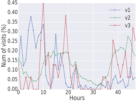
Figure 1 shows three rows of the normalized S in our experiment. The data points were calculated using taxi trajectories. A residential location v1 is easy to identify by rising workday morning and evening visits. The number of visits to a popular shopping location v2 increases at 9am and lasts until midnight. The curve of a sightseeing location v3 even reveals the hours during which it is open (between two daily peaks). This observation is consistent with earlier research suggesting that locations containing large dynamic populations are readily visible in comparatively coarse wireless-traffic analyses [Reades et al., 2007].
In accordance with the observation, to distinguish each location v, we represent all the locations using kt common components E ∈ Rkt×h (also known as bases in Nonnegative Matrix Factorization). As a result, the locations' temporal view-based latent representations Vt ∈ R|V |×kt are learned by the following Nonnegative Matrix Factorization:
where ‖·‖2 denotes the Frobenius norm. The latter two entries of Eq. 1 are regularizers for penalizing the norms of Vt and E. After the first step, the knowledge graph G(V,R) is represented as G(Vt, R = ∅), where R is an empty set.
3.2 Spatial View-based Construction
We capture the spatial influence from Trs, in the second step, by first creating a transition matrix T ∈ R|V |×|V | . Similar to the transition matrix defined in a Markov chain, an entry Ti,j denotes the probability of a transition (movement) from location vi to vj. Creating such a matrix for Trs is straightforward. For each Tr = p1 → p2 → ... → pn, using the longitude and latitude information, we first map it to the locations: Tr′ = v1 → v2 → ... → vm. Then, by aggregating all the Tr′ s, we obtain the initial transition matrix T ′ , the entry T ′ i,j of which records the number of movements vi → vj . Lastly, T is equal to the normalized T ′ .
Given the transition graph T, for each location v, we embed the structured information of T by a factorization of T :
where Vs ∈ R|V |×ks is the embedding matrix, M ∈ Rks×ks is the interaction matrix and ks specifies the number of latent features. Similar to Eq. 1, the latent matrices Vs and M are computed by solving the following optimization function:
Eq. 2 can be regarded as a model for embedding the graph structure. Namely, the latent matrix Vs is an embedding of the locations in a latent component space, where the similarity of locations in this space reflects their similarity in the domain of graph T . M models the interactions of the latent components in this space.
After the second step, the knowledge graph G(V, R) is represented as G([Vt; Vs], T). The locations V are described by concatenating Vt and Vs. For relations R, T is assigned indicating the mutual dependencies among different locations.
3.3 Spatio-temporal View-based Construction
In the third step, we face the challenge of labeling edges on the transition graph T. Given the current knowledge graph G([Vt; Vs], T), although we can observe which locations are tightly related, we do not know why this occurs. In the final step, we perform the relation extraction task in an unsupervised manner. In other words, we try to divide the graph T into several sub-graphs, T1, T2, ..., Tr, each of which represents one kind of relation. The relations can be regarded as different lifestyles (moving patterns) in a city.
Although relation extraction is a extensively investigated research topic [Nickel et al., 2016], to the best of our knowledge, few work have attempted to perform the extraction in an unsupervised manner (i.e., without labeling any edges of T ). Two new methods are proposed in our framework.
(1) Selectional Preference-based Method
In natural language processing, the term selectional preference denotes the tendency of a word to co-occur with words that belong to certain lexical sets. For example, the adjective delicious prefers to modify nouns that denote food. Accordingly, we assume that relations ∀r ∈ (vh, r, vt) also have selectional preferences. Intuitively, a relation r allows only certain location types in its head-argument slot and tail-argument slot. As a result, a selectional preference bridges the observed time series matrix S and transition graph T .
In this method, for each location, we draw a latent vector v ∈ R1×kts . For each relation, we draw a latent vector r ∈ R1×arity(r)∗kts , where function arity(r) returns the number of argument slots of r. Since in our case r is a binary relation (there is a head-argument slot for head location vh and a tailargument slot for tail location vt), arity(r) = 2. Hence, a relation can be represented in a concatenating way: r =< dh, dt >, where d ∈ R1×kts denotes an argument slot.
As a result, measuring the compatibility of a tuple (vh, r, vt) (i.e., the edge weight of T) amounts to summing up the compatibility between the representations of each location (vh, vt) and the corresponding argument slots (dh, dt). Then, we have the following objective function:
where Vts ∈ R|V |×kts records all the locations v and D∗ ∈ R|V |×kts record all the argument slots dh, dt, respectively.
By jointly considering the spatial and temporal influences, i.e., Eq. 4 and Eq. 1, the selectional preference-based relation extraction method minimizes the following function:
where Vts is shared in the first and second entries. After learning, a hierarchical clustering method is utilized for all candidate relations < dh, dt >, dh ∈ Dh; dt ∈ Dt. A cluster corresponds to one kind of relation.
However, in the context of unsupervised learning, we find that the current method is only suitable for 1-to-1 relations. In other words, for an N-to-1 relation r of which the head could be multiple instances, they most likely will be divided into different clusters. Next, an improved method is devised.
(2) Neural Network (NN)-based Method
The most important advantage of this method is that, in addition to the latent variables, the neural network (NN)-based method also learns the objective function rather than assuming it to be fixed. Compared with the fixed Obj1 in Eq. 4, we define the NN-based objective function:
where Vts ∈ R|V |×kts records all the locations; Rts ∈ R|R|×kr records all the relations; I is a latent indexing matrix; C ∈ Rkr×kr is a constant sparsity matrix [PascualMontano et al., 2006]; fΦ(⃗t) denotes a feed-forward NN; W1 ∈ Rn×(2kts+kr) and W2 ∈ Rn×1 , respectively, represent the weights of its first and second layers; n is the number of hidden neurons; Sigmoid() is an element-wise sigmoid function.
For each tuple (vh, r, vt), an indexing vector I(vh,r,vt) ∈ R1×|R| is introduced to specify a relation in R. The sparsity of I(vh,r,vt) is increased as much as possible by introducing a constant sparsity matrix C = (1 - θ)eye(kr) + θ kr ones(kr) [Pascual-Montano et al., 2006], where eye(kr) is an identity matrix of size kr × kr, ones(kr) is a matrix of size kr × kr with all entries of 1s, and θ is the sparsity parameter. When we multiply C with Rts in Eq. 6, to compensate for the loss of sparsity in Rts, I(vh,r,vt) becomes sparse. An extreme example is that, there is only one entry in I(vh,r,vt) close to 1, whereas the other entries approximate 0. The introduction of I allows a relation to have multiple head or tail instances. As a result, this method can accommodate N-to-1, 1-to-N, and N-to-N relations.
Thus, the NN fΦ has 2kts + kr real-valued input units and one real-valued output unit. The first 2kts inputs are headand tail-specific features, respectively, whereas the last kr inputs are relation-specific features. As mentioned above, in addition to learning the latent variables Vts, I, and Rts, this method further learns the objective function, i.e., fΦ.
Similar to Eq. 5, the NN-based method is defined as:
According to the survey [Nickel et al., 2016], feed-forward NNs have already been applied in state-of-the-art supervised relation extraction tasks (e.g., [Van de Cruys, 2014]) and the KV project [Dong et al., 2014]. By observing the context information of head and tail locations (i.e., S), our work goes further by applying an NN in an unsupervised relation extraction task. Because of the NN matrix factorization ensemble, we refer to Eq. 7 as NN matrix factorization. Our method is consistent with the proposal in [Stewart and Ermon, 2016]. That is, for a label-free learning task, we are leveraging prior knowledge (S, T, and selectional preference) to restrict the space of possible functions specifying the hypothesis class (the NNs fΦ with different weights in our case). In this context, our NN matrix factorization provides a new way for encoding prior knowledge into loss functions.
Intuitively, by proposing these two relation extraction methods, two constraints are satisfied: (1) syntactic constraint (Eq. 4 and 6) for eliminating incoherent extractions and (2) lexical constraint (the second entries in Eq. 5 and 7) for constraining certain location types in a relation's head- and tail-argument slots. The final knowledge graph can be represented as G(Vts(1),Rts(1)) and G(Vts(2),Rts(2)), which are learned by Eq. 5 and Eq. 7, respectively.
3.4 An Application
The introduction of this application is two-fold: first, to verify the utility of the learned knowledge graph Gs; and second, to provide a quantitative analysis on Gs.
The application problem can be described as: by observing a part of the user-location attention matrix Xo , we expect to predict the unobserved attention matrix X¬o satisfactorily. In our application, we partition a city into 50 × 50 = 2, 500 grids. Therefore, each grid is a location. By collecting geotagged check-ins, we first construct the user-grid attention matrix X. An entry Xi,j records the attention range (0 to 1) of user ui to a location vj. Detailed information about X is presented in Section 4.
Similar to related work on collaborative filtering, e.g., [Salakhutdinov and Mnih, 2007] [Wang and Blei, 2011], as shown in Algorithm 1, by placing Gaussian priors N(⃗µ, σ2 ) on latent feature vectors, we solve this prediction problem using a generative process.
Algorithm 1 Generative process for attention prediction.
| 1: 2: | for each user ⃗ ui ∈ U do ▷ Stage 1 draw latent user vector ⃗ ui ∼ N(0, σ2U I) |
| 3: 4: | end for for each location ⃗ vj ∈ V do ▷ Stage 2 |
| 5: | draw latent location offset vector ⃗ oj ∼ N(0, σ2V I) draw latent location vector ⃗ vj = ⃗ oj + ⃗ v∗ |
| 6: | j end for |
| 7: | for each user-location pair (⃗ ui, ⃗ vj) ∈ X do ▷ Stage draw the rating Xi,j ∼N(⃗ ui T ⃗ vj , σ2X ) |
| 8: | 3 |
| 9: 10: | end for |
In stage 2, we enrich the latent feature vectors of locations by embedding the knowledge graph. Namely, V ∗ , ∀ ⃗ v∗ j ∈ V ∗ could be Vt, [Vt; Vs], Vts(1), or Vts(2). In the experiments, by comparison, we discuss in detail why our knowledge graph G can significantly improve such an application.
3.5 Latent Variable Learning
Since there is nothing new about the training processes in our framework and application, we briefly describe the training strategies used in the experiments.
We minimize the objective functions Eq. 1, Eq. 3, and Eq. 5 with a gradient decent approach by iteratively optimizing the latent variables Vt, E, Vs, M, Vts, Dh, and Dt. For Eq. 7, we alternate between optimizing the NN weights (i.e., W1 and W2), while fixing the latent features, and optimizing the latent features, while fixing the network weights. Optimization is also carried out by gradient descent on the observed datasets (i.e., S and T ).
For Algorithm 1, the optimization could be carried out by maximizing the log-likelihood [Wang and Blei, 2011], minimizing a sum-of-squared errors function [Salakhutdinov and Mnih, 2007], or using Gibbs sampling. In our experiment, we utilized a previously proposed method [Salakhutdinov and Mnih, 2007] for consistency. Namely, all the learning tasks are conducted in a matrix factorization manner.
4 Experiments
4.1 Dataset Preparation
Constructing S and T . We used the public Beijing taxi trajectory dataset [Yuan et al., 2011], which contains trajectories of 10,357 taxis, to generate the S and T . The total number of GPS points p (see Definition 1) is approximately 15 million. Figure 1 shows some examples of S. Figure 2a shows a taxi's Tr′ (see Section 3.2) in one day on Google Maps. All the Tr′ are aggregated to obtain T ∈ R2500×2500 . Although the other edge weights are close to zero, 35,259 main edges are detected in T .
Constructing X. The user-grid attention matrix is constructed using geo-tagged check-ins collected from Sina Weibo APIs 1 . In total, we obtained a raw dataset consisting of 527,809 users and 1,729,998 check-ins in Beijing in 2015. Then, similar to the CCCF model [Wu et al., 2016], we first conduct a preliminary task of user-region co-clustering to discover like-minded user groups, each of whom has similar interests (i.e., visiting similar regions). After clustering, we calculate each observed entry Xi,j based on the percentage of numbers of check-ins that were uploaded by user group ui in grid vj. Figure 2b shows the percentages of two Xi,js over all the weeks in 2015. Unsurprisingly, because of anomalous events, the percentages fluctuate over time. The value of each observed Xi,j is the average percentage of all the recorded weeks. Finally, we obtain the X of 100 classified user groups and 2,500 grids with 43,069 observed user-grid entries.
4.2 Evaluation Scheme
We randomly divide all the grids associated with each user group into two chunks. One round of validation performs training on one chunk and tests the trained model on the other chunk. The utility of our knowledge graph is evaluated and compared under both sparse (insufficient) and dense (sufficient) training settings, i.e., x = 10%, 30% of the grids are selected as the training chunk, respectively. For each value of x, we repeat the validation five times with different randomly selected training sets. Finally, the average performance is reported for analysis.
1 http://open.weibo.com/wiki/API
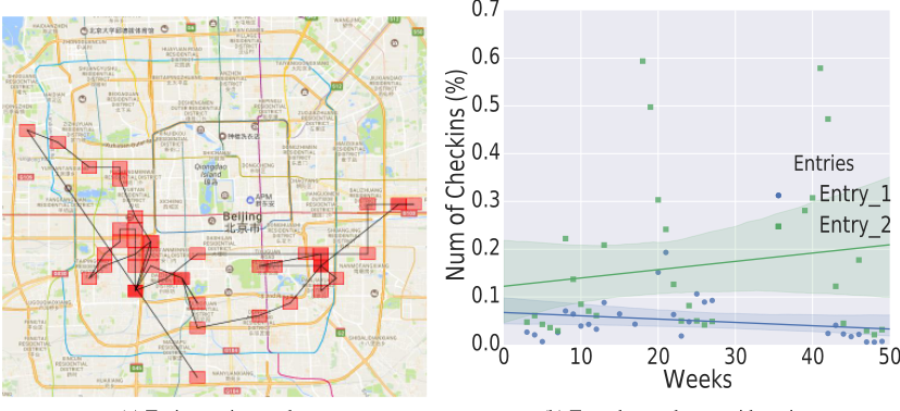
Figure 2: Dataset preparation
Similar to [Wang and Blei, 2011], we used recall as the performance measure because the rating information in X is in the form of implicit feedback (high sparsity) [Hu et al., 2008]. A zero entry in X may be due to the fact that the user group either does not prefer the grid or does not know about it. This complicates the precision of the computation. Because recall only considers the nonzero entries, for each user group we define recall@M as:
where TPs@M (True Positives) is the number of grids to which the user group pays attention in the top M, and TPs@M + FNs@M (False Negatives) is the total number of grids to which the user group pays attention. The reported recall for the entire system is the average recall from all user groups.
4.3 Baselines and Quantitative Comparison
We first list all models included in our comparison as well as the values of their hyperparameters tuned by the grid searchbased method [Hsu et al., 2003]. We named Algorithm 1 the Knowledge Graph based Probabilistic Matrix Factorization (KGPMF).
- KGPMF-none, KGPMF-Vt, KGPMF-Vt&Vs, KGPMF-Vts(1), KGPMF-Vts(2). These five variants are obtained when none, Vt, [Vt; Vs], and Vtss are assigned to V ∗ in Algorithm 1, respectively. When learning the urban movement knowledge graph G, the values of the hyperparameters are: kt = 20; ks = 20; kts = 10; kr = 5; n = 20; λr = 0.01; λs = 1; θ = 0.8.
- GeoMF. A state-of-the-art method for location recommendation [Lian et al., 2014]. By using an influence area vector, GeoMF takes the location-location spatial information into consideration.
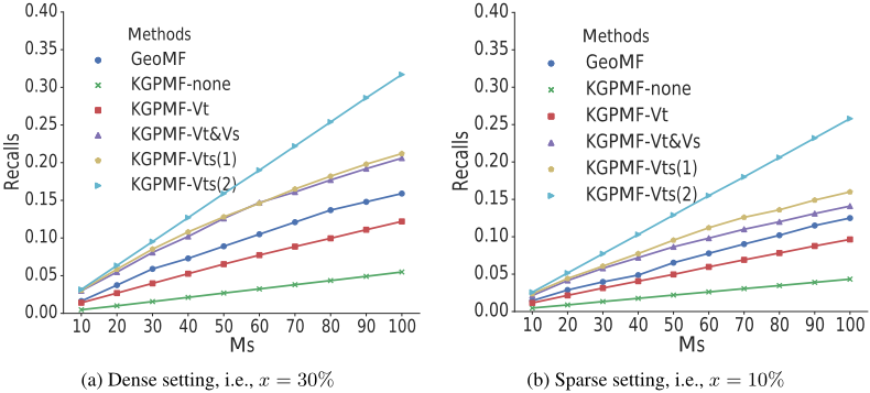
The experimental results are reported in Figure 3. Figure 3a shows the results under a dense setting (i.e., x = 30%), whereas Figure 3b shows the results under a sparse setting (i.e., x = 10%). Overall, the results show that our knowledge graph greatly improves the prediction performance. The details are as follows.
User attention prediction is a challenging problem. The curve of KGPMF-none indicates, without introducing any auxiliary information, that this method performs poorly, especially under a sparse setting.
The spatial information Vs is essential for the prediction. A comparison of the curves of KGPMF-Vt and KGPMF-Vt&Vs shows that KGPMF-Vt&Vs significantly outperformed KGPMF-Vt by an average margin of 3.4% in the sparse setting and 5.8% in the dense setting. On the basis of Eq. 8, when M is small (e.g., M = 10, ..., 100), a margin of 1% is a significant improvement. In conventional collaborative filtering-based recommendation (e.g., for movies), if a user prefers sci-fi movies, given a new sci-fi movie, the model would predict a high score for this user. However, this assumption is not applicable in our case. That is, a user living in residential area A (high attention) rarely pays attention to another faraway residential area B. Hence, in addition to the content features Vt of the locations, the mutual dependencies among them (i.e., Vs) are essential for this type of prediction.
The POI-influence-areas matrix proposed in GeoMF is insufficient. A POI-influence-areas matrix was previously defined [Lian et al., 2014]. For each POI (i.e., rows in the matrix), they assumed the influence areas of the POI to be fixed and have a normal distribution centered at this POI. As a result, important spatial information is lost. For example, a semantic work ↔ home relation [Cho et al., 2011] cannot be embedded when learning. By comparing GeoMF with the other methods shown in Figure 3, it can be further improved. KGPMF-Vts(1) and KGPMF-Vts(2) obtained the highest performance. Compared with KGPMF-Vt&Vs that separately takes temporal and spatial information into consideration, KGPMF-Vts(1) and KGPMF-Vts(2) jointly consider both of them. Several latent semantic relations are detected among the locations. We can regard these relations as lifestyles in a city. For example, office workers may pay more attention to the locations in the work ↔ home relations. Students may pay more attention to the locations in the school ↔ shopping relations. Consequently, when a small training set is used (i.e., the sparse setting), KGPMFVts(1) significantly outperforms KGPMF-Vt&Vs, suggesting that KGPMF-Vts(1) and KGPMF-Vts(2) provide two ways to leverage GPS trajectories into a latent semantic space.
(a) Taxi route in one day
4.4 Knowledge Graph Visualization
Since KGPMF-Vts(2) obtains the best results in our experiment, the Google Maps APIs are utilized on KGPMF-Vts(2) to learn some relation instances, as shown in Figure 4.
Figure 4a shows a shopping like relation between red grids (head) and blue grids (tail). By zooming in on the map, we find that almost all the blue grids are shopping areas. More specifically, Figure 4b shows that there is a shopping mall in A, a plaza in B, a famous shopping street in C and the Times Square in D. Although E is not as well known, we find it has many bank ATMs suggesting it is also a shopping area.
Figure 4c and 4d present two other interesting relation instances. In Figure 4c, our method detected an airport expressway, because of the high similarity among head grids. Figure 4d shows an instance our method learned in the Zhongguancun district. Although the grids in Zhongguancun very likely play multi-roles (e.g., for working, education, shopping, and residency ), a residency-to-education like relation is detected. For example, H contains a university and some research institutes. However, we find that several large universities are missing in this relation. Labeled by F, Tsinghua University is not included. One possible explanation is that, since most of the students and teachers reside on campus (e.g., G, which has many apartments and dormitories), they walk to their learning places. The taxi trajectories cannot characterize such cases. Although only GPS points are used in our framework, the case studies show that our method performed well in terms of learning semantic relations among locations.
5 RelatedWork
Enrichment of latent user features. A number of conventional location recommendation models relying on users' visiting history, geographical influence, temporal influence, etc., have been proposed to infer users' location preferences. For instance, HMM [Kim and Cho, 2013], periodic GMM [Cho et al., 2011], and BPP [Yuan et al., 2014] have been proposed to model individual mobility behavior for preferences inferring. A user preference prediction method investigating the context of the location was proposed [Liu et al., 2016b]. They assumed a user's visit to a location is not only influenced by the set of locations they previously visited, but also by the locations they subsequently visited. Recently, several studies [Wang et al., 2015] [Liu et al., 2016a] focused on predicting the places users are expected to visit next, based on their previously generated content. Nevertheless, these related studies mainly focus on enriching the latent user features, i.e., stage 1 in our Algorithm 1.
Enrichment of latent location features. Few studies have considered the enrichment of latent location features. One reason may be that, in most of the aforementioned POI recommendation models based on the enrichment of latent user features, they assumed that POI categories (i.e., Vt in our case) are observed. However, as mentioned in Section 4.3, this is insufficient. Some initially believed [Yang et al., 2013] that location similarity can also influence recommendation. They constructed a similarity network according to their geodistance and categories. Then, the GeoMF model [Lian et al., 2014] defined a POI-influence-area matrix based on the geodistance. They assumed the influence areas of a POI to have a normal distribution centered at this POI. To the best of our knowledge, the enrichment of latent location features has not been well investigated yet. Our framework is among the first of its kind to systematically construct a knowledge graph G for location oriented enrichment. Not only the categories belonging to the location (i.e., nodes on G) but also the relations among them (i.e., edges on G) are embedded.
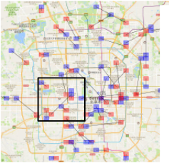
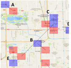
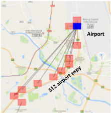
Figure 4: Relation visualization. Red: heads; blue: tails.
Relation extraction. A survey [Nickel et al., 2016] revealed that most of the methods attempting to use machine learning (e.g., TranE [Bordes et al., 2013], TranH [Wang et al., 2014], and TranR [Lin et al., 2015]) are trained on existing knowledge graphs (e.g., Freebase, Wikidata, and YAGO2) in a supervised manner and then used to predict new edges on those graphs. Similar to our methods, we list some latent feature models for comparison. In [Nickel et al., 2012], a tensor factorization based model, RESCAL, is proposed for describing the pairwise interactions of latent features. Recently, several NN-based models were proposed, e.g., [Socher et al., 2013] [Van de Cruys, 2014], to reduce the number of parameters used in RESCAL. NNs can learn to position semantically similar nodes close to each other even if they are not explicitly trained to do this [Mikolov et al., 2013]. For our framework, which is an NN matrix factorization ensemble, we devised a novel NN matrix factorization method for unsupervised relational learning, rather than using supervised graph completion.
6 Conclusion
In this paper, given GPS trajectories, we proposed a novel framework for constructing an urban movement knowledge graph that embeds temporal and spatial information. Two new unsupervised relation extraction methods were devised to learn the relations among nodes on this graph. An application was proposed to present the utility of the knowledge graph. An experiment on a real-world dataset showed significant improvements compared with the baselines. In future, by incorporating additional semantic information (e.g., location categories and city map information), we intend exploring ways to improve the expressiveness of the knowledge graph.
Acknowledgments
This work is partly supported by JSPS KAKENHI (16K12532, 15J01402) and MIC SCOPE (172307001).
@inproceedings{ijcai2017p506,
  title     = {Understanding People Lifestyles: Construction of Urban Movement Knowledge Graph from GPS Trajectory},
  author    = {Zhuang, Chenyi and Yuan, Nicholas Jing and Song, Ruihua and Xie, Xing and Ma, Qiang},
  booktitle = {Proceedings of the Twenty-Sixth International Joint Conference on
               Artificial Intelligence, {IJCAI-17}},
  publisher = {International Joint Conferences on Artificial Intelligence Organization},
  editor    = {Carles Sierra, IIIA-CSIC},
  pages     = {3616--3623},
  year      = {2017},
  month     = {8},
  note      = {Main track},
  doi       = {10.24963/ijcai.2017/506},
  url       = {https://doi.org/10.24963/ijcai.2017/506},
}
TY - CPAPER TI - Understanding People Lifestyles: Construction of Urban Movement Knowledge Graph from GPS Trajectory AU - Zhuang, Chenyi AU - Yuan, Nicholas Jing AU - Song, Ruihua AU - Xie, Xing AU - Ma, Qiang T2 - Proceedings of the Twenty-Sixth International Joint Conference on Artificial Intelligence, IJCAI-17 PB - International Joint Conferences on Artificial Intelligence Organization PY - 2017 SP - 3616 EP - 3623 DO - 10.24963/ijcai.2017/506 UR - https://doi.org/10.24963/ijcai.2017/506 ER -Copied
Machine-readable versions of this paper, for tools and AI agents:





