
NN-kNN for Regression: Accurate Prediction from Interpretable Retrieval
Proceedings of the Thirty-Fifth International Joint Conference on Artificial Intelligence. Main Track. Pages 826-834.
https://doi.org/10.24963/ijcai.2026/93
Keywords
- AI Ethics, Trust, Fairnes: Explainability and interpretability
- Machine Learning: Regression
- Knowledge Representation and Reasoning: Case-based reasoning
- Machine Learning: Trustworthy machine learning
- AI Ethics, Trust, Fairnes: Trustworthy AI
Abstract
Neural Network k-Nearest Neighbor (NN-kNN) was proposed as an interpretable network model that learns feature weights and similarity to retrieve relevant cases for classification. This paper extends it to regression with the goal of generating accurate predictions based on neighboring cases with similar labels. Specifically, we introduce three modular components: an attention mechanism that weights the contribution of retrieved cases, a locality-aware regularizer that favors label-similar neighbors, and an optional case adaptation module that refines the retrieved estimate. Across synthetic and standard tabular regression benchmarks, NN-kNN achieves competitive predictive error against strong baselines (kNN-R, MLKR, and MLPs) while providing cases with similar labels as explanation (later referred as label-similar case). Moreover, NN-kNN supports manual knowledge injection through tuning weights for human-comprehensible features. The result is a simple, general, and interpretable approach to continuous-valued prediction that unifies retrieval, attention, and optional case adaptation within a single neural framework.
- [Aamodt and Plaza, 1994] Agnar Aamodt and Enric Plaza. Case-based reasoning: Foundational issues, methodolog- ical variations, and system approaches. AI Communica- tions, 7(1):39-59, 1994.
- [Bicego and Loog, 2016] Manuele Bicego and Marco Loog. Weighted k-nearest neighbor revisited. In Twenty-Third International Conference on Pattern Recognition (ICPR), pages 1642-1647. IEEE, 2016.
- [Breiman et al., 1984] Leo Breiman, Jerome H. Friedman, Richard A. Olshen, and Charles J. Stone. Classification and Regression Trees. Chapman and Hall/CRC, 1 edition, 1984.
- [Chen et al., 2019] Chaofan Chen, Oscar Li, Daniel Tao, Alina Barnett, Cynthia Rudin, and Jonathan K Su. This looks like that: Deep learning for interpretable image recognition. In Advances in Neural Information Process- ing Systems, volume 32. Curran, 2019.
- [Cortes and Vapnik, 1995] Corinna Cortes and Vladimir Vapnik. Support-vector networks. Machine Learning, 20(3):273-297, 1995.
- [Cover and Hart, 1967] Thomas Cover and Peter Hart. Near- est neighbor pattern classification. IEEE Transactions on Information Theory, 13(1):21-27, 1967.
- [Deng et al., 2025] Kuo Deng, Xiaomeng Ye, Kun Wang, Angelina Pennino, Abigail Jarvis, and Yola Hall. Fully in- terpretable and adjustable model for depression diagnosis: A qualitative approach. The International FLAIRS Con- ference Proceedings, 38(1), May 2025.
- [Doshi-Velez and Kim, 2017] Finale Doshi-Velez and Been Kim. Towards a rigorous science of interpretable machine learning. arXiv preprint arXiv:1702.08608, 2017.
- [Doyle et al., 2006] Dónal Doyle, Padraig Cunningham, and Paul Walsh. An evaluation of the usefulness of explanation in a case-based reasoning system for decision support in bronchiolitis treatment. Computational Intelligence, 22(3- 4):269-281, 2006.
- [Gates et al., 2023] Lawrence Gates, David Leake, and Kait- lynne Wilkerson. Cases are king: A user study of case pre- sentation to explain CBR decisions. In Case-Based Rea- soning Research and Development, ICCBR 2023, pages 153-168. Springer, 2023.
- [Hanney and Keane, 1996] Kathleen Hanney and Mark T. Keane. Learning adaptation rules from a case-base. In Pro- ceedings of the Third European Workshop on Case-Based Reasoning, pages 179-192, Berlin, 1996. Springer.
- [Hastie and Tibshirani, 1986] Trevor Hastie and Robert Tib- shirani. Generalized additive models. Statistical science, 1(3):297-310, 1986.
- [He et al., 2016] Kaiming He, Xiangyu Zhang, Shaoqing Ren, and Jian Sun. Deep residual learning for image recog- nition. In 2016 IEEE Conference on Computer Vision and Pattern Recognition (CVPR), pages 770-778, 2016.
- [Jalali et al., 2017] V. Jalali, D. Leake, and N. Forouzan- dehmehr. Learning and applying case adaptation rules for classification: An ensemble approach. In Proceedings of the Twenty-Sixth International Joint Conference on Ar- tificial Intelligence, pages 4874-4878. International Joint Conferences on Artificial Intelligence, 2017. IJCAI
- [Keane and Kenny, 2019] Mark T. Keane and Eoin M. Kenny. How case-based reasoning explains neural net- works: A theoretical analysis of XAI using post-hoc explanation-by-example from a survey of ann-cbr twin- systems. In Case-Based Reasoning Research and Devel- opment, pages 155-171, Cham, 2019. Springer.
- Kelly et al., ] Markelle Kelly, Rachel Longjohn, and Kolby Nottingham. The uci machine learning repository. https: //archive.ics.uci.edu. Accessed: 2026-04-09. Link
- [Kulis, 2013] Brian Kulis. Metric learning: A survey. Foun- dations and Trends in Machine Learning, 5(4):287-364, 2013.
- [Leake and Ye, 2021] David Leake and Xiaomeng Ye. Har- monizing case retrieval and adaptation with alternating op- timization. In Case-Based Reasoning Research and Devel- opment, pages 125-139, Cham, 2021. Springer.
- [Leake, 1996] David B. Leake. CBR in context: The present and future. In David B. Leake, editor, Case-Based Reason- ing: Experiences, Lessons, and Future Directions, pages 3-30. AAAI Press, Menlo Park, CA, 1996.
- [LeCun et al., 2015] Yann LeCun, Yoshua Bengio, and Ge- offrey Hinton. Deep learning. Nature, 521(7553):436- 444, 2015.
- [Li et al., 2017] Oscar Li, Hao Liu, Chaofan Chen, and Cynthia Rudin. Deep learning for case-based reasoning through prototypes: A neural network that explains its pre- dictions. arXiv preprint arXiv:1710.04806, 2017.
- [Liao et al., 2018] Chieh-Kang Liao, Alan Liu, and Yu- Sheng Chao. A machine learning approach to case adapta- tion. In 2018 IEEE First International Conference on Ar- tificial Intelligence and Knowledge Engineering (AIKE), pages 106-109, 2018.
- [Papernot and Mcdaniel, 2018] Nicolas Papernot and Patrick Mcdaniel. Deep k-nearest neighbors: Towards confident, interpretable and robust deep learning. ArXiv preprint ArXiv:1803.04765, 2018.
- [Rousseeuw and Croux, 1993] Peter J. Rousseeuw and Christophe Croux. Alternatives to the median absolute deviation. Journal of the American Statistical Association, 88(424):1273-1283, 1993.
- [Rudin, 2019] Cynthia Rudin. Stop explaining black box machine learning models for high stakes decisions and use interpretable models instead. Nature Machine Intelligence, 1(5):206-215, 2019.
- [Smyth and Keane, 1998] Barry Smyth and Mark T. Keane. Adaptation-guided retrieval: Questioning the similarity as- sumption in reasoning. Artificial Intelligence, 102(2):249- 293, 1998.
- [The SciPy Community, 2025] The SciPy Community. scipy.stats.median abs deviation. SciPy Documentation (v1.16.2 Manual), 2025. Accessed: 2025-12-26.
- [Weinberger and Tesauro, 2007] Kilian Q. Weinberger and Gerald Tesauro. Metric learning for kernel regression. In Proceedings of the Eleventh International Conference on Artificial Intelligence and Statistics (AISTATS), pages 612-619. PMLR, 2007.
- [Wettschereck et al., 1997] Dietrich Wettschereck, David W. Aha, and Takao Mohri. A review and empirical evaluation of feature weighting methods for a class of lazy learning algorithms, page 273-314. Kluwer Academic Publishers, USA, 1997.
- [Ye et al., 2022] Xiaomeng Ye, David Leake, and David Crandall. Case adaptation with neural networks: Capa- bilities and limitations. In Mark T. Keane and Nirmalie Wiratunga, editors, Case-Based Reasoning Research and Development, pages 143-158, Cham, 2022. Springer.
- [Ye et al., 2024] Xiaomeng Ye, David Leake, Yu Wang, Zi- wei Zhao, and David Crandall. Towards network imple- mentation of CBR: Case study of a neural network K- NN algorithm. In Case-Based Reasoning Research and Development, ICCBR 2024, pages 354-370, Cham, 2024. Springer.
- [Ye et al., 2025] Xiaomeng Ye, David Leake, Yu Wang, and David Crandall. Run like a neural network, explain like k-nearest neighbor. In Proceedings of the Thirty-Fourth International Joint Conference on Artificial Intelligence, IJCAI-25, pages 6857-6865. International Joint Confer- ences on Artificial Intelligence, 2025. IJCAI
- [Zhang et al., 2017] Zhifei Zhang, Yang Song, and Hairong Qi. Age progression/regression by conditional adversarial autoencoder. In IEEE Conference on Computer Vision and Pattern Recognition (CVPR). IEEE, 2017.
References were extracted automatically from the PDF and may contain errors.
Full text extracted automatically from the PDF; figures, tables and equations may differ. The PDF is the version of record.
1 Introduction
Many of today's strongest predictors-including deep neural networks [LeCun et al., 2015], kernel methods such as support vector machines [Cortes and Vapnik, 1995], and supervised metric-learning methods such as MLKR [Weinberger and Tesauro, 2007]-achieve excellent accuracy but can be difficult to interpret. This opacity motivates much work on interpretability and the limits of post-hoc explanations [DoshiVelez and Kim, 2017; Rudin, 2019]. In contrast, classic transparent models such as decision trees [Breiman et al., 1984] and generalized additive models [Hastie and Tibshirani, 1986] provide more direct reasoning traces, but can sacrifice flexibility and predictive power on complex problems.
The k-nearest neighbors (k-NN) algorithm is a classic interpretable method that answers a query by retrieving the k most similar training instances and predicting by majority vote (classification) or (distance-)weighted averaging (regression) [Cover and Hart, 1967]. Viewed through the lens of case-based reasoning (CBR), k-NN performs case-based prediction by solving new problems via retrieval of similar prior cases from memory [Aamodt and Plaza, 1994; Leake, 1996]. In CBR terms, each training example is a case consisting of a problem description x and a solution y. We use this case vocabulary when discussing explanations, but otherwise follow standard ML notation, where x denotes the input features and y the target (class label or real value). We call a retrieved case (xi, yi) a label-similar neighbor for a query (xq, yq) when its label yi provides local support for the query target yq (same class in classification, numerically close in regression). In practice, similarity is typically defined over the inputs xi and xq, even though the ground-truth similarity metric for x-space is often unknown. Human subjects studies have supported the usefulness of similar cases as explanations [Doyle et al., 2006; Gates et al., 2023], and this paper treats similar neighbors as natural case-based explanations.*
A variety of interpretable approaches combine neural representations with example-based explanations [Keane and Kenny, 2019; Li et al., 2017; Chen et al., 2019]. One example is Deep k-Nearest Neighbors (DkNN), which performs kNN lookup in the hidden representations of a pretrained deep model to provide post-hoc explanations and confidence estimates [Papernot and Mcdaniel, 2018]. In contrast, the neural network based k-nearest neighbor (NN-kNN) model [Ye et al., 2025] integrates retrieval and aggregation into the predictor itself, jointly learning a feature extractor, feature importance weights [Wettschereck et al., 1997], case weights [Bicego and Loog, 2016], and a task-specific distance metric. Unlike standard neural models, NN-kNN remains transparent at inference time by retrieving training cases and exposing how they contribute to the output, and it has shown strong performance on classification tasks ranging from tabular data to images and text.
This study considers the major extension of NN-kNN toward regression, which involves a set of challenges detailed in Sec. 3.1. Most notably, NN-kNN, or retrieval-based methods in general, may predict the target label yq accurately by learning to retrieve cases whose target values are far apart and assign them weights such that the weighted combination matches yq. As an extreme example, a model can interpolate a straight line perfectly with only two data points and any query on the line can be calculated as a weighted combination of the two data points. In this setting, the retrieved cases indeed produce accurate results, yet they can be based on poor neighbors for similarity-based explanation: they do not provide locally consistent evidence for the predicted value. Section 4.3 illustrates such misalignment between accuracy and explanation quality arising in practice. This study focuses on learning to retrieve cases that simultaneously provide good predictions and good similarity-based explanations.
* Other forms of case-based explanations (counterfactuals, semifactuals) are not in the scope of this study.
This work makes the following contributions*† :
- NN-kNN for regression via attention-weighted label aggregation. We extend NN-kNN beyond classification by replacing majority voting with an attentionweighted aggregation of retrieved numeric labels, enabling continuous-valued prediction while preserving case-based explanations through per-neighbor weights.
- Retrieval of label-similar cases for regression. We improve retrieval in NN-kNN regression by penalizing attention assigned to top-K neighbors whose labels deviate beyond a preset tolerance, encouraging retrieval of a set of cases whose label is similar to the query target.
- Optional label adaptation via case differences. To reduce reliance on imperfect retrieval, our method optionally adapts retrieved labels for the query using a learned case-difference heuristic case adaptation mechanism.
- NN-kNN learns semantically meaningful feature weights and allows knowledge injection by manual tuning. Feature weights provide a straightforward indication of a feature's relative importance (the higher the more important). NN-kNN for regression learns feature weights that reflect ground-truth feature importance. Users can also manually adjust learned feature weights to steer retrieval and prediction toward expertprovided judgments of feature importance. Therefore, NN-kNN provides a simple mechanism for injecting domain knowledge.
2 RelatedWork
2.1 Original NN-kNN
The original neural network k-nearest neighbor model (NNkNN) formulates the k-NN retrieval-and-vote pipeline as a differentiable neural computation graph, enabling end-to-end learning of similarity and aggregation mechanisms [Ye et al., 2024; Ye et al., 2025].
Given a query xq and a case base {(xi, yi)}Ni=1 , NN-kNN applies a learnable feature extractor ϕ(·) and performs retrieval in the resulting embedding space, z = ϕ(x) (ϕ can be an identity function if no feature extraction is needed). The distance dqi between query xq and case xi is computed as
* As permitted by IJCAI policy, the authors used an LLM to assist with formatting, such as table and equation typesetting, and language polishing. All scientific content was written by the authors.
† All code and additional results can be found at https://github. com/Heuzi/NNkNN-Regression.
where wi is the effective feature weight for case i. We parameterize wi by mixing a small set of global weight patterns {w(s) }Ss=1 using a case-specific mixture vector αi ∈ RS . Intuitively, {w(s) }Ss=1 represents S feature-importance patterns, and αi determines how strongly each pattern contributes to case i's feature weights:
This parameter-efficient formulation interpolates between global weighting (S = 1) and local weighting as S increases, and is hence named glocal feature weighting.
Case activation is determined by
where bi is a learnable case bias and τ is a temperature parameter. Activations are aggregated using learned case weights ci. For classification, evidence for class k is computed as
NN-kNN is inherently interpretable: predictions are constructed directly from retrieved cases, and the learned parameters reveal how features and cases contribute to decisions.
2.2 CBRAdaptation
In case-based reasoning (CBR) for regression, retrieval alone is often insufficient, since the retrieved cases rarely match the query's target label exactly. Small but meaningful differences in the problem description can correspond to systematic shifts in the target value. A solution is to apply an adaptation step that adjusts retrieved solutions to better fit the query.
The case difference heuristic (CDH) was introduced to learn adaptation rules from case pairs by attributing solution differences to the pairs' problem differences [Hanney and Keane, 1996; Jalali et al., 2017; Liao et al., 2018]. Most relevant here is a neural network-based case difference heuristic method, NN-CDH [Ye et al., 2022]. Using the notation in Sec. 2.1, let zq = ϕ(xq) and zi = ϕ(xi) be embeddings for the query and a retrieved case. NN-CDH defines a neural adapter gψ(·) that takes the case context zi and the case difference ∆zqi = zq - zi, and outputs an adjustment to the retrieved label yi,
However, because zq = (zq - zi) + zi, the adapter can reconstruct the query embedding and potentially predict the target directly, bypassing adaptation. To prevent this embedding leakage, we modify NN-CDH to condition on the retrieved label yi rather than the context embedding zi.
3 NN-kNN for Regression
3.1 Challenges for Retrieval-Based Regression
A basic tenet of CBR is that similar problems have similar solutions. In classification, nearby inputs often share the same label, so a majority vote from retrieved neighbors typically supports the predicted class. In regression, the target is continuous and predictions are formed by attention- or distanceweighted averaging over retrieved neighbors. This presents two challenges in regression:
(1) Inaccuracy from similarity misalignment. Retrieval selects neighbors based on input-space similarity, but accurate prediction requires neighbors that are also label-similar. This motivates learning (or carefully designing) a similarity measure that aligns input-space similarity with label similarity. Metric learning is extensively studied for classification [Kulis, 2013], but is less emphasized in regression, with fewer dedicated approaches (e.g., MLKR [Weinberger and Tesauro, 2007]). For example, on the CARS dataset in Tab. 1, MLKR and NN-kNN (SOFTMAX) learn a similarity metric yet underperform their non-trainable counterpart, weighted k-NN. This suggests that the learned metric can become misaligned with label similarity (e.g., due to overfitting and/or an unfavorable inductive bias), reducing retrieval quality and downstream accuracy.
(2) Accurate but dissimilar label mixtures. A retrievalbased predictor can match the query target by mixing neighbors with widely separated labels, yielding accurate predictions but weak similarity-based explanations. As an extreme illustration, any point on a straight line can be interpolated as a weighted combination of the line's two endpoints, even if neither endpoint is locally similar to the query. We observe this behavior for "NN-kNN (SOFTMAX) w/o Lld" in Tab. 2: it achieves strong predictive accuracy (best after adaptation) while retrieving the least similar neighbors under the hidden ground-truth distance metric.
3.2 NN-kNN for Regression
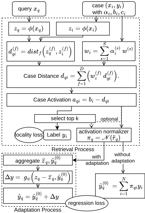
This study builds a retrieval-based model to accurately predict continuous labels and explain with label-similar cases. Moreover, only a small set of cases should be activated. Fig. 1 shows the overall architecture. The following describes the modifications to NN-kNN from Sec. 2.1.
Attention Computation and Normalization. An attention mechanism assigns a relevance weight to each retrieved case and enables prediction by a weighted average of their labels. For a query q, we compute the distance dqi to each training case i using Eq. (1), and define a simplified case activation,
where bi ∈ R is a learnable case bias that represents the default activation of case i. This formulation allows cases to activate over different query regions and avoids committing to a neighborhood of fixed K samples as in traditional k-NN.
We convert these activations into an attention distribution using a global normalizer,
where aq = (aq1, . . . , aqN) is the activation vector over all N cases, τ > 0 is a temperature hyperparameter, and Norm(·) can be instantiated as softmax or a sparse simplex normalizer such as sparsemax. Softmax yields a dense distribution over cases, whereas sparse normalizers can assign exact zero mass to many cases, resulting in a smaller set of influential neighbors. In either case, this replaces original independent gating (Eq. (3)) with a normalization in which all cases compete for probability mass and the resulting weights form a proper distribution (πqi ≥ 0, ∑i πqi = 1).
The regression prediction is obtained by attentionweighted averaging of retrieved labels,
Optional NN-CDH Adaptation. The attention-weighted average ˆ y(0) q can be inaccurate when the target value lies near the tail of the label distribution (e.g., outliers or extreme values), where even the most relevant retrieved cases may remain systematically biased above or below yq. To improve accuracy beyond what retrieval alone can provide, we introduce an optional NN-CDH adaptation module that adjusts the retrieved prediction using the discrepancy between the query and the retrieved neighborhood.
When adaptation is enabled, the model first forms an aggregate retrieved case (prototype) in representation space, together with its corresponding aggregate label,
where zi denote the learned embeddings of case i (Sec. 2.1). The model then applies an NN-CDH adaptation network gψ that operates on the case problem difference and the retrieved context label, producing an additive solution correction,
The final adapted prediction is
Because adaptation can "fix" errors downstream, when retrieval and adaptation are trained together, retrieval becomes less selective and may converge to less label-similar neighborhoods [Smyth and Keane, 1998; Leake and Ye, 2021]. Although not a primary focus here, we mitigate this issue with staged training. We first train retrieval alone (without adaptation) to establish a label-similar neighborhood structure, then freeze retrieval and train NN-CDH to perform targeted label adjustment on the fixed retrieved neighborhoods.
3.3 Training Objectives
In NN-kNN, the embedding function ϕθ, the distance computation parameters (w, α) (Sec. 2.1), the case biases {bi}Ni=1 , and (when enabled) the NN-CDH adapter gψ are trained endto-end by backpropagation under the following objectives.
Regression loss. This is amean squared error loss that measures the error of the final prediction,
Case-bias regularization. The learnable case-specific bias bi in Eq. (5) allows each training case to adjust its baseline tendency to be retrieved. Without regularization, these biases may grow and dominate the distance term, leading to degenerate retrieval behavior (e.g., a small set of cases receiving consistently high attention regardless of the query). We therefore add an ℓ2 penalty on the bias parameters,
where N is the number of training cases.
Locality Regularization. Beyond minimizing prediction error, we encourage the attention mechanism in Eq. (6) to concentrate on label-similar neighbors, i.e., retrieved cases whose labels do not deviate excessively from the query target. We apply the locality penalty to the normalized attention mass over the retrieved set. Let Iq = TopK(πq1, . . . , πqN) be the indices of the top-K attended cases for query q, and define
so that ∑i∈Iq ˜πqi = 1.
We normalize label deviation using the median absolute deviation (MAD), a robust alternative to standard deviation that is less sensitive to outliers. To obtain a standarddeviation-like scale under mild assumptions, we apply the normal-consistency correction σy = 1.4826 · MAD, where 1.4826 = 1/Φ-1 (0.75) [Rousseeuw and Croux, 1993; The SciPy Community, 2025]. Using a dimensionless tolerance ϵ > 0, we penalize label distances beyond ϵ,
where α ∈ {1, 2} controls the penalty growth.
Training objective. The overall training objective is a weighted sum of the losses defined above,
4 Evaluation
We evaluate NN-kNN for regression through four experiments. The first compares predictive performance against strong baselines on standard tabular datasets. The second tests performance on high-dimensional inputs using an image dataset with frozen feature extraction. The third uses a synthetic dataset with a known ground-truth feature weighting to assess whether NN-kNN's explanations-feature weights, retrieved cases, and case biases-align with ground truth. The fourth is a case study illustrating how manual feature tuning can incorporate externally-provided preferences.
Hyperparameters and training settings. We experiment with both softmax and sparsemax as the case activation normalizer Norm (Eq. (6)), with temperature τ = 1.0 controlling the sharpness of the case-attention distribution. We use K = 40 for the normalized attention subset Iq in the locality regularizers (Eq. (13)-(14)). In the label-distance loss (Eq. (14)), we set the tolerance ϵ = 0.1 and exponent α = 2, and weight the locality terms with λld = 0.1 in the full objective (Eq. (15)). We train the model with a batch size of 64 using Adam, with learning rates of 10-3 for the feature extractor ϕ and the glocal feature-weighting module, and 3 × 10⁻⁴ for the case biases; Training is conducted for up to 7000 epochs, with early stopping applied based on validation performance, using a patience of 80 epochs. NN-CDH is first pretrained on 5N randomly sampled case pairs (N is the number of training cases) and then incorporated into NNkNN. We next train the retrieval components and freeze them, and subsequently fine-tune NN-CDH within the full model.
Preprocessing and evaluation metric. We perform a random 80/20 train-validation split and compute normalization statistics on the training split only. Input features are standardized per dimension using the training-set mean and standard deviation, and the same transformation is applied to validation features. We also standardize y using the training-set mean and standard deviation. For reporting, we convert predictions back to the original target scale via ˆ yraw = ˆ y σy +µy and report RMSE in the raw target units.
Computational experiments are organized into the following subsections, each guided by a specific hypothesis or experimental goal.
4.1 Performance on Tabular Datasets
Hypothesis: NN-kNN achieves comparable or lower RMSE than weighted k-NN, MLKR, and MLP on standard regression datasets.
We compare these models on standard regression benchmarks from scikit-learn (California Housing, Diabetes) and the UCI Repository [Kelly et al., ] (Abalone, Body Fat, Bike Sharing, Wine Quality, Airfoil, Cars/Automobile, Student Performance, Yacht, Energy Efficiency). The weighted k-NN baseline retrieves the k nearest training samples under Euclidean distance in x-space (or z-space if feature extraction is involved) and predicts by an inverse-distance weighted average. We set k = 5 based on preliminary trials and keep it fixed across datasets to maintain a simple, uniform baseline comparison. We include the MLP as a strong parametric neural baseline that does not perform retrieval, to assess whether NN-kNN remains competitive with standard black-box predictors. We include MLKR (Metric Learning for Kernel Regression) as a regression-oriented metric-learning baseline. MLKR learns a Mahalanobis distance so that nearby points in the learned space support accurate kernel-weighted prediction, making it a close point of comparison to NN-kNN's learned similarity and attention-weighted prediction.
All results are produced with one shared configuration across datasets (see Tab. 1). Considering the interaction between normalizer, locality, and adaptation, modest datasetspecific tuning would likely yield further gains. The key findings are:
- Overall competitiveness. Across most datasets, NNkNN is competitive with strong baselines and typically outperforms weighted k-NN and MLKR. This highlights the benefit of learning representations, feature weights, and case importance end-to-end.
- Softmax vs. sparsemax performance is datasetdependent. Different datasets favor different aggregation behaviors. For example, Student Performance results consistently favor softmax variants, suggesting that smoother averaging can be beneficial when the target function is not strongly locally clustered.
- Softmax interacts less robustly with locality and adaptation. While sparsemax performs well on datasets with strong local structure (e.g., Cars, Yacht, Energy Efficiency), softmax variants are more brittle in combination with other components. First, softmax may
conflict with locality regularization on locally structured datasets (e.g., California Housing, where softmax+locality degrades relative to softmax-only). Second, adaptation can further worsen performance when retrieval is already misaligned: for instance, on California Housing, softmax+locality+adaptation underperforms softmax+locality, suggesting that here adaptation may amplify upstream retrieval errors rather than correcting them.
- Failure scenarios concentrate in specific configurations, not the framework as a whole. When NNkNN underperforms vanilla weighted k-NN (e.g., Cars), the underperformance is largely confined to particular softmax configurations; sparsemax resolves these cases. This suggests a normalizer-regularizer interaction issue rather than an inherent limitation of NN-kNN.
4.2 Performance on High-Dimensional Inputs
Hypothesis: With a frozen feature extractor for highdimensional inputs, NN-kNN matches an MLP head in predictive performance while retrieving label-similar neighbors as case-based explanations.
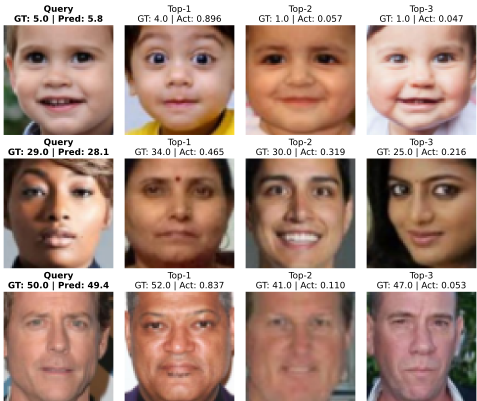
To test NN-kNN on high-dimensional inputs while avoiding confounds from representation learning, we evaluate a setting where all models operate on the same fixed feature vectors. Concretely, we perform age prediction on the UTKFace dataset [Zhang et al., 2017], where each image is resized to 64×64 with three color channels and then encoded to an embedding extracted from the penultimate layer of a pretrained frozen ResNet18 [He et al., 2016]. We adopt the same train-validation split as in the other datasets. To facilitate training, we randomly select 4,000 samples from the training-set to construct the case base. The learning rate is set to 5 × 10⁻⁴ for the glocal feature-weighting module and
| Model | CH | Di | Ab | BF | BS | WQ | AF | Cars | SP | Y | EE | UTK |
|---|---|---|---|---|---|---|---|---|---|---|---|---|
| Weighted k-NN | 0.634 | 61.85 | 2.24 | 0.013 | 111.51 | 0.634 | 2.38 | 12683.68 | 2.43 | 10.50 | 2.30 | 12.98 |
| MLP | 0.494 | 57.10 | 2.05 | 0.010 | 45.40 | 0.646 | 2.51 | 15763.32 | 1.48 | 4.52 | 1.38 | 11.68 |
| MLKR | 0.466 | 59.70 | 2.15 | 0.012 | 52.31 | 0.596 | 2.44 | 16447.38 | 1.70 | 3.32 | 1.19 | 12.43 |
| NN-kNN (softmax), pure | 0.586 | 58.46 | 2.14 | 0.011 | 71.86 | 0.579 | 2.05 | 13194.01 | 1.41 | 3.24 | 0.942 | 12.60 |
| + adaptation | 0.535 | 57.68 | 2.08 | 0.010 | 62.64 | 0.578 | 1.89 | 11755.02 | 1.34 | 4.50 | 1.38 | 12.04 |
| + locality | 0.665 | 58.51 | 2.16 | 0.011 | 72.04 | 0.577 | 2.08 | 13642.72 | 1.48 | 8.86 | 0.896 | 12.71 |
| + locality + adaptation | 0.903 | 57.35 | 2.07 | 0.011 | 63.72 | 0.576 | 1.98 | 11637.63 | 1.37 | 6.65 | 1.26 | 12.03 |
| NN-kNN (sparsemax), pure + adaptation | 0.445 | 70.31 | 2.22 | 0.014 | 46.92 | 0.594 | 1.64 | 10935.63 | 1.92 | 1.48 | 0.544 | 14.85 |
| 0.438 | 64.06 | 2.12 | 0.012 | 46.32 | 0.589 | 1.58 | 10017.56 | 1.61 | 1.21 | 0.546 | 13.31 | |
| + locality | 0.453 | 70.26 | 2.22 | 0.014 | 47.67 | 0.594 | 1.71 | 9966.15 | 1.80 | 1.49 | 0.477 | 14.95 |
| + locality + adaptation | 0.441 | 64.82 | 2.16 | 0.012 | 46.87 | 0.589 | 1.65 | 9923.38 | 1.54 | 1.01 | 0.501 | 13.22 |
1×10⁻⁴ for the case biases. Models are trained for up to 300 epochs with early stopping using a patience of 15 epochs.
Results. The result is reported in the UTK column of Table 1. NN-kNN remains close to MLP, while retaining its case-based explanation interface (see Fig. 2). In this experiment, NN-kNN is trained to retrieve age-similar cases, not necessarily cases that are visually similar in human-salient aspects such as race or gender. We deliberately use a simple regression objective to keep the comparison with baselines fair and focused on the prediction mechanism itself; incorporating additional objectives for human-salient attributes is an important future direction.
4.3 Explanation fromLearned Parameters
Hypothesis: NN-kNN learns semantically meaningful parameters, producing explanations that reflect the underlying ground truth.
We use a synthetic regression dataset with known (but hidden) feature and case importance to test whether NN-kNN's learned feature weights and case biases recover the generating structure, and whether its retrieved neighbors support similarity-based explanations under the ground-truth metric.
Specifically, we generate a linear regression dataset with additive Gaussian noise. The dataset consists of 3000 samples with 5 features, each drawn independently from a standard normal distribution. The target variable is generated as
where w∗ = [2.5, -1.7, 0.0, 0.9, 3.2]⊤ represents the true underlying feature weights, and ϵ ∼ N(0, 1.02 ) is Gaussian noise. Cases with lower importance have more noise.
Feature Weights Learned. NN-kNN learns feature weights consistent with the ground truth (normalized w∗ : [0.301, 0.205, 0.000, 0.108, 0.386]): softmax learns [0.282, 0.230, 0.000, 0.171, 0.318] and sparsemax learns [0.311, 0.197, 0.046, 0.125, 0.321], correctly emphasizing the relative importance between all weights while keeping w3 near zero. Note that NN-kNN's feature weights are constrained to be nonnegative because they parameterize a distance metric; therefore, they should align with the magnitudes (not the signs) of the ground-truth coefficients.
Nearest Neighbors Found. We study the extent to which different NN-kNN and baseline models retrieve similar neighbors suitable for explanation. Because the synthetic dataset provides ground-truth feature weights, we can directly evaluate retrieval quality against the underlying similarity structure. We compute the mean ground-truth distance of the top K=5 retrieved cases under the weighted ℓ2 metric induced by w∗ . Specifically, for a query xq and retrieved neighbor xi, we define
and report the mean d∗ over the top-K neighbors.
We compare NN-kNN with (i) a weighted-by-distance kNN regressor operating in the original input space and (ii) a multilayer perceptron (MLP) regressor. Because the MLP does not include a built-in retrieval mechanism, we approximate its "implicit" neighbors by extracting penultimate-layer representations for all samples and retrieving the nearest training points under Euclidean distance in that representation space. (iii) We also include an oracle k-NN that retrieves neighbors by label distance, providing an upper bound on retrieval quality. Predictive performance is measured by validation RMSE. As shown in Table 2, NN-kNN achieves competitive RMSE while retrieving neighbors that are closer to the query under the ground-truth metric.
LearnedCase Biases. Because the labels include Gaussian noise ϵ ∼ N(0, 1), some training cases are noisier and can introduce confusion. We quantify this with a case randomness score ri = |yi - x⊤i w∗ |, the absolute deviation between the observed label yi and its noise-free counterpart. We observe a moderate negative correlation between case randomness and the learned case bias (Pearson r = -0.359), suggesting that NN-kNN tends to correctly downweight noisier cases.
The Effect of Sparsemax and Locality Loss In this experiment, we noticed that NN-kNN using either softmax or sparsemax can achieve low prediction error. Adaptation can further improve the error. We also notice that when using softmax without locality regularization, even if NN-kNN is accurate, it tends to activate far away cases. This corresponds to our earlier discussion in Sec. 3.1.
| Model | RMSE | Mean d∗ |
|---|---|---|
| NN-kNN (softmax) w/o Lld after adaptation | 0.9711 0.9603 | 1.3719 |
| NN-kNN (sparsemax) w/o Lld after adaptation | 1.1907 1.0440 | 0.299 |
| NN-kNN (softmax) after adaptation | 0.9854 0.9672 | 0.2853 |
| NN-kNN (sparsemax) after adaptation | 1.1674 1.0460 | 0.3006 |
| Weighted k-NN | 1.3189 | 0.3284 |
| MLP | 0.9638 | 0.4216 |
| Oracle k-NN (y) | 0.0148 | 0.2402 |
In summary, the synthetic dataset results show that for this data, NN-kNN learns feature weights and case biases that align with the ground truth and achieves accurate predictions by retrieving similar neighbors. In contrast, although the MLP attains similar prediction error to NN-kNN, it induces neighbors much farther from the true target under the ground-truth metric, offering weaker support for explanation.
4.4 Manual FeatureWeight Tuning
Previous work [Deng et al., 2025] applied NN-kNN to depression screening and demonstrated that the model supports manual feature weight tuning for mental health practitioners to align model behavior with their domain judgment (e.g., which factors are important for depression). Qualitative evidence suggested that this interaction was useful and interpretable, but most real-world settings lack an objective ground truth for feature importance, making it difficult to quantify the effect of feature weight tuning.
Building on this research direction, we examine the hypothesis: When initialized with manually specified feature weights, NN-kNN can refine them through training while approximately preserving the user-specified weighting.
We construct a synthetic regression dataset (n = 1500) from latent factors s1, s2 ∼ N(0, 1):
with ηj ∼ N(0, 0.052 ) and
Thus x0 measures s1 and (x1, x2) are redundant for s2. To isolate feature weights learning and manual edits, we use sparsemax NN-kNN without NN-CDH or locality regularization, learning a single global feature-weight vector w ∈ R3 (Tab. 3).
In Stage A, we impose a misspecified prior by freezing w0 = w1 = 0 during training. At convergence, the model relies entirely on w2, resulting in poor predictive performance.
| Stage | w0 | w1 | w2 | MSE / R2 |
|---|---|---|---|---|
| A | 0.000 | 0.000 | 0.312 | 0.5285 / 0.4814 |
| B.1 | 0.000 | 0.000 | 0.318 | 0.5290 / 0.4809 |
| B.2 | 0.000 | 0.117 | 0.213 | 0.5361 / 0.4740 |
| C.1 | 0.101 | 0.055 | 0.057 | 0.0096 / 0.9906 |
| C.2 | 0.425 | 0.169 | 0.187 | 0.0092 / 0.9909 |
In Stage B.1, we initialize from the Stage A checkpoint, unfreeze w1 and continue training. This produces no meaningful improvement: the learned weights remain close to Stage A, suggesting that the model does not substantially shift weight from w2 to w1 once it has committed to one of the redundant sensors. In Stage B.2, we simulate expert intervention by manually increasing w1 and suppressing w2, reflecting a user preference for one redundant feature over the other. After retraining, the model assigns more weight to w1 than in B.1, while achieving essentially the same error as Stages A and B.1. This shows that NN-kNN can absorb externally supplied feature preferences and retain them through optimization.
In Stage C.1, we initialize from Stage B.2 and unfreeze w0, allowing all feature weights to adapt freely. The model recovers the intended structure, assigning substantial weight to w0 and achieving near-perfect predictive performance. Finally, in Stage C.2, we start from Stage B.2 again but first manually nudge w0 toward its ground-truth value; the resulting performance is comparable to C.1, indicating that feature edits aligned with the ground-truth do not hinder convergence.
Overall, this experiment illustrates that NN-kNN supports feature-level manual tuning in a transparent and controllable manner. This suggests that edits to feature weights performed by a human would have predictable effects on both model behavior and performance, and could either guide or constrain learning depending on when and how they are applied.
5 Conclusion
NN-kNN for regression produces transparent predictions as an attention-weighted aggregation of retrieved labels. It learns a similarity metric with case- and feature-weights, making each neighbor's contribution explicit and directly interpretable. Across our regression benchmarks, NN-kNN achieves performance competitive with strong baselines while retaining case-based explanations.
A future direction is to extend this case-based transparency beyond supervised regression. In particular, we plan to investigate NN-kNN as a value/policy component in reinforcement learning agents for game playing, where each action can be accompanied by retrieved episodes as an explicit rationale. A second direction is a human subject study to quantify human satisfaction with provided explanations such as label-similar cases and the effectiveness of feature weight tuning.
Acknowledgments
We thank the members of the DeepCBR group at Indiana University Bloomington for their collegial support and exchange of ideas. Ye is supported by Summer Scholarship Stipend (SS 24-25-03) from Berry College.
Contribution Statement
Authors are listed by the extent of their contributions. Ye was involved in all aspects of this project, including writing, code implementation, experiments, logistical planning, team effort organization, and paper submission. Wang was heavily involved in most code implementation, parameter fine-tuning, and all computational experiments; the UTKFace experiment was done by Wang. Leake provided regular consultations on ideas, designs, project direction, and experimental results and was heavily involved in the writing and editing of the article. Crandall provided regular consultations on the ideas, project direction, and paper reviewing. Both Leake and Crandall led the research group DeepCBR at Indiana University Bloomington. Abhieyighan and McGowan assisted in literature search and preliminary experiments.
@inproceedings{ijcai2026p93,
  title     = {NN-kNN for Regression: Accurate Prediction from Interpretable Retrieval},
  author    = {Ye, Xiaomeng and Wang, Yu and Leake, David and Crandall, David and Abhieyighan, Great and McGowan, Mereck},
  booktitle = {Proceedings of the Thirty-Fifth International Joint Conference on
               Artificial Intelligence, {IJCAI-26}},
  publisher = {International Joint Conferences on Artificial Intelligence Organization},
  editor    = {Diego Calvanese},
  pages     = {826--834},
  year      = {2026},
  month     = {8},
  note      = {Main Track},
  doi       = {10.24963/ijcai.2026/93},
  url       = {https://doi.org/10.24963/ijcai.2026/93},
}
TY - CPAPER TI - NN-kNN for Regression: Accurate Prediction from Interpretable Retrieval AU - Ye, Xiaomeng AU - Wang, Yu AU - Leake, David AU - Crandall, David AU - Abhieyighan, Great AU - McGowan, Mereck T2 - Proceedings of the Thirty-Fifth International Joint Conference on Artificial Intelligence, IJCAI-26 PB - International Joint Conferences on Artificial Intelligence Organization PY - 2026 SP - 826 EP - 834 DO - 10.24963/ijcai.2026/93 UR - https://doi.org/10.24963/ijcai.2026/93 ER -Copied
Machine-readable versions of this paper, for tools and AI agents:





