
ExLipBaB: Exact Lipschitz Constant Computation for Piecewise Linear Neural Networks
Proceedings of the Thirty-Fifth International Joint Conference on Artificial Intelligence. Main Track. Pages 753-761.
https://doi.org/10.24963/ijcai.2026/85
Keywords
- Machine Learning: Robustness
- Machine Learning: Adversarial machine learning
- AI Ethics, Trust, Fairnes: Safety and robustness
Abstract
It has been shown that a neural network's Lipschitz constant can be leveraged to derive robustness guarantees, to improve generalizability via regularization or even to construct invertible networks. Therefore, a number of methods varying in the tightness of their bounds and their computational cost have been developed to approximate the Lipschitz constant for different classes of networks. However, comparatively little research exists on methods for exact computation, which has been shown to be NP-hard. Nonetheless, there are applications where one might readily accept the computational cost of an exact method. These applications could include the benchmarking of new methods or the computation of robustness guarantees for small models on sensitive data. Unfortunately, existing exact algorithms restrict themselves to only ReLU-activated networks, which are known to come with severe downsides in the context of Lipschitz-constrained networks. We therefore propose a generalization of the LipBaB algorithm to compute exact Lipschitz constants for arbitrary continuous piecewise linear neural networks and p-norms. With our method, networks may contain traditional activations like ReLU or LeakyReLU, activations like GroupSort or the related MaxMin and FullSort, which have been of increasing interest in the context of Lipschitz-constrained networks, or other piecewise linear functions like MaxPool.
- [Anil et al., 2019] Cem Anil, James Lucas, and Roger Grosse. Sorting Out Lipschitz Function Approximation. In Proceedings of the 36th International Conference on Ma- chine Learning, pages 291-301. PMLR, May 2019.
- [Behrmann et al., 2019] Jens Behrmann, Will Grathwohl, Ricky T. Q. Chen, David Duvenaud, and Joern-Henrik Ja- cobsen. Invertible Residual Networks. In Proceedings of the 36th International Conference on Machine Learning, pages 573-582. PMLR, May 2019.
- [Bhowmick et al., 2021] Aritra Bhowmick, Meenakshi D'Souza, and G. Srinivasa Raghavan. LipBaB: Com- puting Exact Lipschitz Constant of ReLU Networks. In Igor Farkaš, Paolo Masulli, Sebastian Otte, and Stefan Wermter, editors, Artificial Neural Networks and Machine Learning -ICANN 2021, pages 151-162, Cham, 2021. Springer International Publishing.
- [Chen et al., 2019] Ricky T. Q. Chen, Jens Behrmann, David K Duvenaud, and Joern-Henrik Jacobsen. Residual Flows for Invertible Generative Modeling. In Advances in Neural Information Processing Systems, volume 32. Cur- ran Associates, Inc., 2019.
- [Cisse et al., 2017] Moustapha Cisse, Piotr Bojanowski, Edouard Grave, Yann Dauphin, and Nicolas Usunier. Par- seval Networks: Improving Robustness to Adversarial Ex- amples. In Proceedings of the 34th International Confer- ence on Machine Learning, pages 854-863. PMLR, July 2017.
- [Cortez et al., 2009] Paulo Cortez, António Cerdeira, Fer- nando Almeida, Telmo Matos, and José Reis. Model- ing wine preferences by data mining from physicochem- ical properties. Decision Support Systems, 47(4):547-553, November 2009.
- [Diep, 2012] Nguyen Hong Diep. Efficient Implementation of Interval Matrix Multiplication. In Kristján Jónasson, editor, Applied Parallel and Scientific Computing, pages 179-188, Berlin, Heidelberg, 2012. Springer.
- [Ducotterd et al., 2024] Stanislas Ducotterd, Alexis Goujon, Pakshal Bohra, Dimitris Perdios, Sebastian Neumayer, and Michael Unser. Improving Lipschitz-Constrained Neural Networks by Learning Activation Functions. Journal of Machine Learning Research, 25(65):1-30, 2024.
- [Fanaee-T and Gama, 2014] Hadi Fanaee-T and Joao Gama. Event labeling combining ensemble detectors and back- ground knowledge. Progress in Artificial Intelligence, 2(2):113-127, June 2014.
- [Fazlyab et al., 2019] Mahyar Fazlyab, Alexander Robey, Hamed Hassani, Manfred Morari, and George Pappas. Ef- ficient and Accurate Estimation of Lipschitz Constants for Deep Neural Networks. In Advances in Neural Informa- tion Processing Systems, volume 32.
- Curran Associates, Inc., 2019.
- [Gehr et al., 2018] Timon Gehr, Matthew Mirman, Dana Drachsler-Cohen, Petar Tsankov, Swarat Chaudhuri, and Martin Vechev. Ai 2: Safety and robustness certification of neural networks with abstract interpretation. In Security and Privacy (SP), 2018 IEEE Symposium on, 2018.
- [Gendron and Crainic, 1994] Bernard Gendron and Teodor Gabriel Crainic. Parallel Branch-And-Bound Algorithms: Survey and Synthesis. Operations Research, 42(6):1042-1066, 1994.
- [Gorokhovik et al., 1994] V. V. Gorokhovik, O. I. Zorko, and G. Birkhoff. Piecewise affine functions and polyhedral sets. Optimization, 31(3):209-221, January 1994.
- [Goujon et al., 2024] Alexis Goujon, Arian Etemadi, and Michael Unser. On the number of regions of piecewise linear neural networks. Journal of Computational and Ap- plied Mathematics, 441:115667, May 2024.
- [Gouk et al., 2021] Henry Gouk, Eibe Frank, Bernhard Pfahringer, and Michael J. Cree. Regularisation of neu- ral networks by enforcing Lipschitz continuity. Machine Learning, 110(2):393-416, February 2021.
- [Hanin and Rolnick, 2019] Boris Hanin and David Rolnick. Deep ReLU Networks Have Surprisingly Few Activation Patterns. In Advances in Neural Information Processing Systems, volume 32.
- Curran Associates, Inc., 2019.
- [Huster et al., 2019] Todd Huster, Cho-Yu Jason Chiang, and Ritu Chadha. Limitations of the Lipschitz Con- stant as a Defense Against Adversarial Examples. In Carlos Alzate, Anna Monreale, Haytham Assem, Al- bert Bifet, Teodora Sandra Buda, Bora Caglayan, Brett Drury, Eva García-Martín, Ricard Gavaldà, Irena Koprin- ska, Stefan Kramer, Niklas Lavesson, Michael Madden, Ian Molloy, Maria-Irina Nicolae, and Mathieu Sinn, edi- tors, ECML PKDD 2018 Workshops, pages 16-29, Cham, 2019. Springer International Publishing.
- [Johnston, 2016] Nathaniel Johnston. How to compute hard- to-compute matrix norms. https://njohnston.ca/2016/01/ how-to-compute-hard-to-compute-matrix-norms/, 2016. Accessed: 2024-05-22. Link
- [Jordan and Dimakis, 2020] Matt Jordan and Alexandros G Dimakis. Exactly Computing the Local Lipschitz Constant of ReLU Networks. In Advances in Neural Information Processing Systems, volume 33, pages 7344-7353.
- Curran Associates, Inc., 2020.
- [Lee, 2004] Jon Lee. A First Course in Combinatorial Opti- mization. Cambridge Texts in Applied Mathematics. Cam- bridge University Press, Cambridge, 2004.
- [Li et al., 2019] Jianlin Li, Jiangchao Liu, Pengfei Yang, Liqian Chen, Xiaowei Huang, and Lijun Zhang. Ana- lyzing Deep Neural Networks with Symbolic Propagation: Towards Higher Precision and Faster Verification. In Bor- Yuh Evan Chang, editor, Static Analysis, pages 296-319, Cham, 2019. Springer International Publishing.
- [Pauli et al., 2023] Patricia Pauli, Dennis Gramlich, and Frank Allgöwer. Lipschitz constant estimation for 1D con- volutional neural networks. In Proceedings of The 5th Annual Learning for Dynamics and Control Conference, pages 1321-1332. PMLR, June 2023.
- [Pauli et al., 2024] Patricia Pauli, Aaron J. Havens, Alexan- dre Araujo, Siddharth Garg, Farshad Khorrami, Frank Allgöwer, and Bin Hu. Novel Quadratic Constraints for Extending LipSDP beyond Slope-Restricted Activations. In The Twelfth International Conference on Learning Rep- resentations, 2024.
- [Pintore and Després, 2024] Moreno Pintore and Bruno De- sprés. Computable Lipschitz Bounds for Deep Neural Net- works, October 2024. arXiv:2410.21053 [cs].
- [Rump, 2012] Siegfried M. Rump. Fast interval matrix mul- tiplication. Numerical Algorithms, 61(1):1-34, September 2012.
- [Shi et al., 2022] Zhouxing Shi, Yihan Wang, Huan Zhang, J. Zico Kolter, and Cho-Jui Hsieh. Efficiently Computing Local Lipschitz Constants of Neural Networks via Bound Propagation. Advances in Neural Information Processing Systems, 35:2350-2364, December 2022.
- [Stargalla et al., 2025] Moritz Stargalla, Christoph Hertrich, and Daniel Reichman. The Computational Complexity of Counting Linear Regions in ReLU Neural Networks.
- In D. Belgrave, C. Zhang, H. Lin, R. Pascanu, P. Ko- niusz, M. Ghassemi, and N. Chen, editors, Advances in Neural Information Processing Systems, volume 38, pages 125970-125988.
- Curran Associates, Inc., 2025.
- [Szegedy et al., 2014] Christian Szegedy, Wojciech Zaremba, Ilya Sutskever, Joan Bruna, Dumitru Erhan, Ian Goodfellow, and Rob Fergus. Intriguing properties of neural networks, February 2014. arXiv:1312.6199 [cs].
- [Tanielian and Biau, 2021] Ugo Tanielian and Gerard Biau. Approximating Lipschitz continuous functions with GroupSort neural networks. In Proceedings of The 24th International Conference on Artificial Intelligence and Statistics, pages 442-450. PMLR, March 2021.
- [Tao et al., 2022] Qinghua Tao, Li Li, Xiaolin Huang, Xi- angming Xi, Shuning Wang, and Johan A. K. Suykens. Piecewise linear neural networks and deep learning. Na- ture Reviews Methods Primers, 2(1):42, June 2022.
- [Tsuzuku et al., 2018] Yusuke Tsuzuku, Issei Sato, and Masashi Sugiyama. Lipschitz-Margin Training: Scalable Certification of Perturbation Invariance for Deep Neural Networks. In Advances in Neural Information Processing Systems, volume 31.
- Curran Associates, Inc., 2018.
- [Virmaux and Scaman, 2018] Aladin Virmaux and Kevin Scaman. Lipschitz regularity of deep neural networks: analysis and efficient estimation. In Advances in Neural Information Processing Systems, volume 31.
- [Wang, 2022] Yuan Wang. Estimation and Comparison of Linear Regions for ReLU Networks. In Proceedings of the Thirty-First International Joint Conference on Artifi- cial Intelligence, volume 4, pages 3544-3550, July 2022. IJCAI
- [Warwick et al., 1994] Nash Warwick, Sellers Tracy, Talbot Simon, Cawthorn Andrew, and Ford Wes. Abalone, 1994. Published: UCI Machine Learning Repository.
- [Weng et al., 2018a] Lily Weng, Huan Zhang, Hongge Chen, Zhao Song, Cho-Jui Hsieh, Luca Daniel, Duane Boning, and Inderjit Dhillon. Towards Fast Computation of Cer- tified Robustness for ReLU Networks. In Proceedings of the 35th International Conference on Machine Learning, pages 5276-5285. PMLR, July 2018.
- [Weng et al., 2018b] Tsui-Wei Weng, Huan Zhang, Pin-Yu Chen, Jinfeng Yi, Dong Su, Yupeng Gao, Cho-Jui Hsieh, and Luca Daniel. Evaluating the Robustness of Neural Networks: An Extreme Value Theory Approach. In Inter- national Conference on Learning Representations, 2018.
- [Zhang et al., 2024] Zeyu Zhang, Khandaker Asif Ahmed, Md Rakibul Hasan, Tom Gedeon, and Md Zakir Hossain. A Deep Learning Approach to Diabetes Diagnosis. In Ngoc Thanh Nguyen, Richard Chbeir, Yannis Manolopou- los, Hamido Fujita, Tzung-Pei Hong, Le Minh Nguyen, and Krystian Wojtkiewicz, editors, Recent Challenges in Intelligent Information and Database Systems, pages 87- 99, Singapore, 2024. Springer Nature.
References were extracted automatically from the PDF and may contain errors.
Full text extracted automatically from the PDF; figures, tables and equations may differ. The PDF is the version of record.
1 Introduction
In recent years, various methods have been developed that require the computation or approximation of a neural network's (NN's) Lipschitz constant. As the Lipschitz constant quantifies a NN's maximum change in output to small changes in input, a core application is the quantification of a NN's robustness to adversarial examples [Szegedy et al., 2014; Cisse et al., 2017; Tsuzuku et al., 2018; Weng et al., 2018a]. Furthermore, it can be used for regularization [Gouk et al., 2021] and the construction of invertible networks and Residual Normalizing Flows [Behrmann et al., 2019; Chen et al., 2019]. Unfortunately, an exact computation of the Lipschitz constant is NP-hard, which was proven in the case of ReLU networks and the ||.||2-norm [Virmaux and Scaman, 2018]. The majority of research in the field therefore focuses on scalable methods for increasingly tight approximations of the Lipschitz constant [Fazlyab et al., 2019; Weng et al., 2018b; Shi et al., 2022; Pintore and Despr´es, 2024]. Newly proposed methods usually come with certain theoretical guarantees and are also benchmarked on example networks, ideally with a known true Lipschitz constant. To our knowledge, there are currently only two approaches that are able to exactly compute this true constant for non-constructed examples: LipMIP [Jordan and Dimakis, 2020] and LipBaB [Bhowmick et al., 2021]. LipMIP assumes that the ||.||1 or ||.||∞ vector norms are used to define the Lipschitz constant, proposing a generalization to norms which they call "linear". The LipBaB algorithm works for arbitrary p-norms. However, both methods are only applicable to NNs using the ReLU activation. In the context of Lipschitz-constrained NNs, ReLU is however seen with increasing skepticism as authors have proven inapproximability results for layerwise-constrained ReLU-networks [Huster et al., 2019] and raised issues of diminishing gradients for deep networks [Anil et al., 2019].
In practical applications in which the Lipschitz constant only needs to be computed once, like robustness analyses [Pauli et al., 2023] of NNs working with sensitive (small) data (e.g. [Zhang et al., 2024]), which would benefit from an exact computation, as well as in benchmarks mimicking such applications, we therefore argue that there is a need for more general exact computation algorithms to obtain best possible benchmarks and robustness bounds. Even in cases where other activation functions could theoretically be expressed as ReLU-networks, this would result in a sharp increase in computational cost due to increased network size and existing methods would nonetheless have to be adapted to residual networks [Pauli et al., 2024]. We therefore propose in this paper a generalization of the LipBaB algorithm [Bhowmick et al., 2021], which we call Extended LipBaB (ExLipBaB) 1 and which is able to compute the exact local and global Lipschitz constant w.r.t. arbitrary p-norms for any continuous piecewise linear NN . ExLipBaB is therefore in particular also applicable to networks using the GroupSort activation or the related FullSort and MaxMin, which are of particular interest in the field of Lipschitz constraints [Anil et al., 2019; Pauli et al., 2024]. Networks may also include general continuous piecewise linear functions like MaxPool or learned spline activations [Tao et al., 2022; Ducotterd et al., 2024]. Like [Bhowmick et al., 2021], we leverage the Branch-andBound framework to split the input space of piecewise linear NNs into local regions on which the Lipschitz constant can be easily computed. This framework results in an exponential runtime in the worst case but a faster runtime in most practical applications, as not all possible regions will actually have to be evaluated. In cases where running our algorithm to completion would be computationally infeasible, it can be stopped at any time and still deliver a hard upper and lower bound for the Lipschitz constant for a highly flexible class of NNs and arbitrary p-norms.
1 Supplementary material, including the code for our experiments can be found under: https://github.com/tsplittg/ExLipBaB Code.
2 Preliminaries
We first define the following [Jordan and Dimakis, 2020]:
Definition 1. The Lipschitz norm of a function
f : (Rd , ||.||p) → (Rm, ||.||q) over an open set Ω ⊂ Rd is defined as:
.
If this supremum exists and is finite, f is called Lipschitz continuous on Ω.
For better readability, we will usually omit the subscripts p, q and p → q. Also, as is common, we will use the term Lipschitz constant when referring to the Lipschitz norm. If the set Ω is equal to the entire space Rd , this is often referred to as the global Lipschitz constant. In the more general case in which Ω is an arbitrary open subset, L(f, Ω) is referred to as the local Lipschitz constant [Jordan and Dimakis, 2020; Bhowmick et al., 2021]. This should not be confused with the mathematical concept of local Lipschitz continuity.
Many approximation approaches, like the basic layerwise approximation [Gouk et al., 2021] or LipSDP [Fazlyab et al., 2019; Pauli et al., 2024] only aim at computing the global Lipschitz constant. LipMIP [Jordan and Dimakis, 2020] on the other hand is able to exactly compute the local Lipschitz constant w.r.t. "linear" norms, whereas the LipBaB approach [Bhowmick et al., 2021] is able to exactly compute the local and global constant w.r.t. arbitrary p-norms; both algorithms are however only applicable to ReLU networks.
For our generalization of the LipBaB approach, we assume that all functions contained in our NN are continuous piecewise linear (PWL) [Tao et al., 2022; Gorokhovik et al., 1994]: Definition 2. Let Ω ⊂ Rd1 , then a function α : Ω → Rd2
is called PWL if there exists a set {P1, . . . , Pk} of polyhedra (we will always assume convex polyhedra) with interiors P ◦ i such that:
- ⋃ki=1 Pi = Ω and P ◦ i ̸= ∅ ∀i = 1, . . . , k
- iii) For all i = 1, . . . , k, the function α restricted to Pi, is an affine function, i.e. there exist T i ∈ Rd2×d1 , ti ∈ Rd2 such that α|Pi (x) = T ix + ti .
- ii) P ◦ i ∩P ◦ j = ∅ for all i ̸= j
In the following sections, we will always assume that we are working with a neural network f : Rd0 → RdL of the form:
where eachWi is an affine functionWi(x) =Wix+wi corresponding to a linear layer and each αi is a continuous PWL function. One can easily see that the assumption that the linear and PWL layers alternate comes without loss of generality, as we can simply either pad layers with the identity function or join layers (concatenations of affine/PWL functions are again affine/PWL).
NNs based on PWL activations are commonplace in modern machine learning. An overview over the concept can be found in [Tao et al., 2022]. We prove in the supplementary material that componentwise PWL activations like ReLU, LeakyReLU or ParametricReLU (with a slope learned during training) as well as GroupSort (and the related FullSort and MaxMin) satisfy definition 2. A similar argument for the MaxPool function can be found in [Gehr et al., 2018].
For the ReLU activation in d dimensions, a full decomposition of the input space into linear regions would have 2d polyhedron elements. For use in our algorithm, we will therefore use an equivalent decomposition, where the activation state is only fixed for a subset of neurons in each region. This transfers the approach of [Bhowmick et al., 2021] into the general PWL setting:
Remark 1. Let Ω ⊂ Rd1 , then a function α : Ω → Rd2 is called PWL if there exists a set {Q1, . . . ,Q˜k } of polyhedra such that for every neuron n ∈ {1, . . . , d2}, there exists a subset In ⊂ {1, . . . ˜ k}, such that:
- ⋃i∈In Qi = Ω
- for all i ∈ In, there exist T ni ∈ R1×d1 , tni ∈ R, such that πn ◦ α|Qi (x) = T nix + tni is an affine function, where πn is the projection onto the n-th vector element.
2.1 Lipschitz Constant and Jacobian
It is well known that the Lipschitz constant of a linear function A(.) + b : (Rd , ||.||p) → (Rm, ||.||q) equals the induced matrix norm ||A||p→q := maxx̸=0 ||Ax||q ||x||p . Such matrix norms are comparatively easy to compute for common p and q [Johnston, 2016]. Our goal is therefore to reduce the computation of L(f, Ω) to computing the maximum over all matrix norms in the PWL decomposition of f:
Theorem 1. Let α : (Rd1 , ||.||p) → (Rd2 , ||.||q) be a PWL function. Using the notation from definition 2, the following holds:
The proof of this theorem is very similar to the arguments used in [Bhowmick et al., 2021] and therefore not discussed in detail here - we instead refer to the supplementary material. Essentially, we use a result from [Jordan and Dimakis, 2020] to relate the Lipschitz constant of f to the supremum over the norm of its generalized (Clarke) Jacobian over Ω. Then, we show that only differentiable points need to be considered for this supremum, which are exactly the points in the interior of polyhedra Pi in the notation of definition 2.
Algorithm 1 Overview ExLipBaB
Input: Network f, input polyhedron Ω, approximation
factor θOutput: Tuple (glb, gub); global lower- and upper bound
for L(f, Ω) where gub ≤ θ· glb 1: initial activation pattern←SymProp(Ω, f) 2: initial subproblem ρI ←SubProblem(Ω, . . . ) 3: ρI.Lub ←LipschitzBounds(ρI, . . . ) 4: initialize glb, gub← (0, ρI.Lub) 5: initialize: ϱ ←maxHeap([ρI]) 6: if ˜l == L+1 then 7: glb← ρI.Lub //trivial case 8: end if 9: while gub > θ· glb do 10: ρ′ ← argmaxρ∈ϱ(ρ.Lub) 11: ϱ ← ϱ\{ρ′ } 12: (new subproblems, glb) ←Branch(ρ′ , . . . ) 13: ϱ ← (ϱ ∪ new subproblems ) 14: gub←maxρ∈ϱ ρ.Lub 15: end while 16: return (glb, gub)3 Methodology
In theorem 1, we have reduced the computation of L(f,Ω) to the discrete optimization problem ρI : maxi∈S ||T i ||, with S := {1, . . . , k} the finite index set of all polyhedra Pi in the PWL decomposition of the NN f. Like [Bhowmick et al., 2021], we follow the standard branch-and-bound (BnB) framework to recursively solve this problem. A high-level overview of our algorithm is given in Algorithm 1.
At the core of our algorithm is the set ϱ of active subproblems, each representing a discrete optimization problem over a subset Sρ ⊆ S. We will impose that the input space associated with each ρ ∈ ϱ in Rd0 is always a polyhedron. We follow [Lee, 2004], and describe the three main components of our BnB algorithm:
- Bounding ρ ∈ ϱ with good upper bounds, which is described in section 3.3
- Branching a subproblem ρ ∈ ϱ into new subproblems ρ′ with Sρ′ ⊆ Sρ, such that an optimal solution for any ρ′ is also an optimal solution to ρ, see section 3.4
- An efficient method to obtain lower bounds, see section 3.2
The set ϱ is initialized as ϱ = {ρI}, where the bounding of ρI is described in section 3.2. Our algorithm then maintains a global upper bound (gub) and global lower bound (glb) over all subproblems. In the recursive step, the subproblem ρ ∈ ϱ with the largest upper bound is removed from ϱ and branched into subproblems associated with smaller regions of the input space. For each smaller subproblem ρ′ , an upper bound is computed and the gub is updated accordingly. Also, if the upper bound is smaller than the glb, we discard ρ′ (fathomed by bounds). If we can solve ρ′ exactly, we also return a lower bound LB and update the glb as max(glb, LB); afterwards, we again discard ρ′ (fathomed by optimality). If a ρ′ is not discarded by either of these rules, it is appended into ϱ. The algorithm runs until all subproblems are fathomed or until θ · glb ≥ gub for a pre-determined approximation factor θ. Either way, termination is guaranteed and if the algorithm is run to completion, the true maximum is found [Lee, 2004; Gendron and Crainic, 1994]. In the following sections, we describe the components of our algorithm in more detail.
3.1 Abstract Interpretation
At creation, each subproblem ρ is assigned an associated polyhedron Ωρ ⊂ Ω in input space. We consider ρ exactly solvable, if f, constrained to Ωρ, is fixed affine, in which case we only have to compute a single matrix norm to solve ρ. To determine whether f is fixed affine on Ωρ, we compute a list of neurons in f which we call ⋆-neurons, which potentially take different activation states in Ωρ. For this, we leverage the concept of abstract interpretation [Gehr et al., 2018]. Given a layer index 1 ≤ l ≤ L, we wish to find an abstract transformer f # l that transforms the polyhedron Ωρ of possible inputs into f to a dl-dimensional polyhedron f # l (Ωρ) of potentially possible pre-activation states in the lth layer. We can then intersect f # l (Ωρ) with all polyhedra in the PWL decomposition of αl. If for a neuron n, there are at least two polyhedra with non-empty intersection with f # l (Ωρ), such that the activation state of n on these polyhedra is different, then we call n a ⋆-neuron.
An abstract transformer f # l can simply be constructed by concatenating abstract transformers of the individual layers of f. For linear layers, the affine transformation of a polyhedron automatically is a polyhedron. For PWL layers αm, the polyhedron of potential pre-activations is intersected with all polyhedra of the PWL decomposition of αm. Then, each intersection is transformed with the corresponding fixed affine state of αm and finally a polyhedron is constructed that is a superset of all these smaller transformed polyhedra. This process is described in more detail in [Gehr et al., 2018] (note that what the authors call "CAT" functions is simply a subclass of PWL functions).
For each layer, we record the minimum and maximum value of the activation weights and biases for each neuron over all non-empty intersections in an interval matrix [Λ]l and an interval vector [λ]l respectively. In other words, these interval matrices (vectors) contain at each entry an interval of plausible values for the activation state at the given entry (see e.g. [Rump, 2012]). We also record with ˜l the first layer of f in subproblem ρ which contains ⋆-neurons.
In abstract interpretation, one often restricts the type of abstract sets to be boxes or zonotopes instead of polyhedra. This drastically improves performance at the cost of looser bounds, which is why the initialization algorithm which we describe in section 3.2 uses the box region for all newly added abstract variables. Note that the tightness of the bounds in the initial symbolic propagation only affects initialization and does not alter the exactness of the final result.
3.2 Initialization
To initialize the set of subproblems ϱ, an activation pattern and an upper bound have to be computed for the initial subproblem and an initial glb has to be specified. In [Bhowmick et al., 2021], the initial glb is simply set to zero and updated only when a subproblem is solved exactly. We instead propose to evaluate the norm of the Jacobian of f in a few randomly chosen points in Ω. This is computationally inexpensive and, due to theorem 1, results in a hard lower bound if f is differentiable in all chosen points. Theoretically, the probability of accidentally choosing a non-differentiable point is zero [Jordan and Dimakis, 2020]; in practice, due to floating point inaccuracy, it is only very small. Also, the case of accidentally selecting non-differentiable points could easily be prevented algorithmically. We test this non-trivial lower bound initialization in practice in section 4.3.
For the computation of the initial activation pattern, we adapt the SymProp algorithm from [Bhowmick et al., 2021] to the general PWL setting. This algorithm makes use of symbolic propagation [Li et al., 2019] and does not propagate explicit polyhedra through f as was described in section 3.1. Instead, it propagates linear relations whenever possible. This approach can help to reduce the overapproximation resulting from the well-known dependeny problem. The idea is to represent the state of a neuron as an abstract linear equation of input variables if the activation state of f is fixed affine on that neuron. If the activation state of the neuron isn't fixed, a new abstract input variable is introduced to preserve linear relations in deeper layers. We detail the propagation through the first layer, the other layers follow recursively:
For f, we assume the notation of equation (1). The input is represented as a d0-dimensional symbolic variable that takes values in a polyhedron Ωρ. Let C, c be the half space representation of Ωρ, i.e. Ωρ = {x ∈ Rd0 : Cx ≤ c} and define ˜ B := W1, ˜b := w1. Denote also by Ai, ai the half space constraints of the i-th polyhedron Pi in the PWL decomposition of α1 according to remark 1. Formally, all of these variables need an additional index because they are iterated upon in the recursion, but to improve readability we will slightly abuse notation and omit these indices. We then first determine which activation states α1 possibly takes. For this, we set
where stack(.) represents the vertical stacking of two matrices. It holds that
Let I be the set of indices of the polyhedra that fulfill either side of equation (3). The candidate set of ⋆-neurons in the current layer is then the set of neurons whose state is determined in at least two Pi, i ∈ I. In order to reduce the number of unnecessary splits, we however only classify a neuron as ⋆-neuron, if the activation states differ in these polyhedra. Using the notation from remark 1, we demand that either T ni or tni differ between at least two polyhedra. This check is necessary for certain decompositions and less so for others; for example, in the full PWL decomposition of a d-dimensional ReLU activation according to definition 2, any neuron is fixed active in 2d-1 polyhedra whereas we describe an alternative decomposition in the supplementary material where it is only fixed active in exactly one polyhedron.
Let J be the index set of ⋆-neurons at the current layer. For a neuron n /∈ J , we denote by T ni and tni the n-th row and n-th bias element of the unique activation state of α on n respectively. To propagate the symbolic linear relations on non-⋆-neurons through α1, we can simply apply these affine functions. For ⋆-neurons however, we can no longer maintain linear relationships. Like [Li et al., 2019] suggests, we therefore concretize the post-activation bounds of these neurons and add new symbolic variables to the input set that take values within these bounds. Thereby, we hope to maintain linear relations in following layers.
Let j ∈ J and denote by min(j),max(j) the minimal and maximal post-activation value of this ⋆-neuron. We then form ̂Ωρ := Ωρ × (×j∈J [min(j),max(j)]), which is a polyhedron of dimensionality ̂ d0 := d0 + |J |.
Let T be the d1 × d0 matrix and t be the d1-dimensional vector, whose rows, respectively entries, are zero for ⋆- neuron indices and equal to T ni , respectively tni , for neurons with a unique activation state. We then define a new vector ̂b of length d1 and a matrix ̂ B of shape d1 × ̂ d0, by setting ̂b := T · ˜b + t and, for (n, j) ∈ d1 × ̂ d0:
It is easy to see that the propagation via these matrices is an overapproximation of the propagation by α1 in the sense that α1 ◦ W1(Ωρ) ⊂ ̂ B · ̂Ω + ̂b. In the previously mentioned slight abuse of notation, we now close the recursive loop by renaming
While recursively continuing this propagation through the entire network, we save the indices and layers of the ⋆-neurons and the layer ˜l ∈ {1, . . .L} in which the first ⋆-neuron appears. We also compute two lists of interval matrices: [Λ] and [λ]. They contain, for each layer, an interval matrix and an interval vector which each contain as their entries an interval defined by the maximum and minimum entries over all possible linear activation states T ni and tni . These interval matrices are necessary for section 3.3. Note that, unlike in [Bhowmick et al., 2021], the interval matrices we obtain in our algorithm are not necessarily diagonal matrices.
3.3 Lipschitz Bounds
To compute the upper Lipschitz bound for an individual subproblem ρ with associated region Ωρ, we first assume that the activation state of f on Ωρ, in the form of ˜l, as well as [Λ] and [λ], has already been computed. These computations are either done in SymProp or FFilter (see section 3.4 below).
As ˜l is the first layer index with ⋆-neurons, the function ˜ f := (W˜l ◦ α˜l-1 ◦ · · · ◦W1)|Ωρ is affine (where we define WL+1 =Id). We can therefore easily compute the Jacobian J ˜ f of ˜ f through a simple matrix product.
If ˜l = L+ 1, i.e. if the network contains no ⋆-neurons on Ωρ, then f = ˜ f and we simply return ||J˜ f ||.
If ˜l ≤ L, we leverage interval matrix multiplication to construct a matrix which is in each component absolutely larger than Jf . In interval matrix multiplication, the product of two interval matrices [A], [B] is again an interval matrix which, as its components, contains intervals that overapproximate all possible results A·B, where A and B have entries from the intervals of [A] and [B]. This product can be computed through a brute force combinatorial approach which is intuitive but lengthy, which is why we refer to [Diep, 2012] for a more comprehensive introduction.
We now define an initial interval matrix [J˜l ] := [J˜ f , J˜ f ] and recursively compute
for l = ˜l + 1, . . . , L. Notice that, even though we allow both our linear and activation layers to include biases, their presence does not matter for the computation of the (approximation of the) Jacobian. Finally, we set U as the (dL × d0)- matrix with entries Uij := max(|[Jij]L|, |[Jij]L|).
If now x ∈ Ωρ is an arbitrary point in which f is differentiable, then there exists a polyhedron P ⊂ Ωρ on which f is fixed affine, such that x ∈ P ◦ . Then, for each layer l, the PWL function αl takes a fixed affine form Alx + bl with A ∈ [Λ]l, where we slightly abuse notation to denote by "∈" a realization of the interval matrix. Then, due to the properties of interval matrix multiplication,
Therefore, by definition of U, it holds for all i, j that Jf (x)ij ≤ Uij .
The following lemma therefore proves that ||U|| is a hard upper bound for L(f, Ωρ):
Lemma 1 ([Bhowmick et al., 2021, Lemma 2]). Let U be a matrix of the same size as the Jacobian Jf(x) of a PWL function f. If U is such that supx∈Ω |Jf(x)ij| ≤ Uij for all i, j and all points x in which f is differentiable, then Lp→q(f, Ω) ≤ ||U||p→q.
In [Bhowmick et al., 2021], this lemma is only proven for p = q. However, as their proof easily transfers to the general case, we only discuss it in the supplementary material.
3.4 Branching
After having described the bounding step, we now describe the branching step of the recursion in more detail. At a given iteration, given the current set of subproblems ϱ, we first remove the subproblem ρ with the maximal upper bound from ϱ. We assume that [Λ], [λ] and ˜l have been computed for ρ in an earlier iteration and that ρ is associated with a polyhedron Ωρ. As ρ will not have be solved, we can get the index n of the first ⋆-neuron in layer ˜l. We then iterate through all polyhedra Pi in the PWL decomposition of α˜l with respect to neuron n as defined in remark 1. Similar to our approach in equation (3), we stack the half-space constraints of Ωρ with the constraints of Pi, propagated back to the input dimension, to obtain a new polyhedron Qi. This propagation is possible because, on ρ, f is fixed affine in all layers before ˜l. If the intersection defined by the stacking of constraints is not empty, we initialize a new subproblem ρi associated with Qi in input space. Since Qi ⊂ Ωρ, we know that the Lipschitz constant of each new subproblem is not larger than that of ρ, meaning that a feasible solution of the new subproblems is also a feasible solution of ρ. Also, per definition, each ρi has strictly fewer ⋆-neurons than ρ as the state of n is fixed. We then update the activation states of ρi (see below) and compute the upper (lower) bounds. Afterwards, each new subproblem is either terminated according to the rules at the beginning of section 3 or added to ϱ, which completes the recursion.
Note that iterating through all polyhedra in a decomposition according to remark 1 can be intuitively understood as setting the activation state of only that neuron (plus some others that automatically get set with it, depending on the PWL function). One hopes that the constriction enforced by setting one neuron also results in the fixing of others. One could also use a decomposition as in definition 2 to force this, but this would imply a drastic increase in the number of necessary polyhedra. The advantage would be that we would be certain that layer ˜l is fixed in all newly created subproblems.
FFilter After the branching step, we run a feasibility filter, which combines the LinProp and FFilter algorithms of [Bhowmick et al., 2021], to check whether we have also implicitly set the state of other neurons. We multiply the first (˜l - 1) layers, on which f is linear, into one linear function and then, starting with layer ˜l, check whether the other layers contain ⋆-neurons or not. Also, [Λ]˜l and [λ]˜l are updated. If a layer does not contain ⋆-neurons, its linear state is multiplied with the propagated linear function and ˜l increased by one. We terminate this process if we encounter a layer with ⋆-neurons. Activation states of deeper layers are not updated.
3.5 Convergence Guarantee
After the algorithm has been run - either to completion or until a fixed approximation quality has been reached - the global upper and lower bounds are returned. If the algorithm is run to completion, these two bounds match and are an exact solution to the maximization problem in equation (2):
Lemma 2. The solved subproblem with the greatest upper bound is an optimal solution of the maximization problem, i.e. its upper bound equals the true Lipschitz constant of f.
This is a standard result from Branch-and-Bound theory [Lee, 2004]. We also mention that our algorithm suffices the theorem of [Gendron and Crainic, 1994]:
Proof. As we only implemented an elimination via upper and lower bounds, we only have to check the first two convergence assumptions of [Gendron and Crainic, 1994]. Firstly, our algorithm only returns a lower bound for a subproblem ρ, if ρ contains no ⋆-neurons. In such a case, the lower bound equals the true Lipschitz constant of f constrained to Ωρ and is therefore a feasible solution to the original problem. Secondly, a subproblem is solved if and only if its upper and lower bound have been computed and are equal.
In particular, if the initial input space is set as Ω = Rd0 , our method computes the true global Lipschitz constant.
| ReLU | GroupSort | |||
|---|---|---|---|---|
| L(f )[std] | time | L(f)[std] | time | |
| Layerwise | 3.12 [0.50] | 0.00s | 1.62 [0.32] | 0.00s |
| ExLipBaB | 1.15 [0.20] | 0.03s | 1.01 [0.24] | 0.03s |
| LipSDP | 1.62 [0.32] | 3.63s | 1.30 [0.30] | 0.00s |
4 Experiments
In this section, we apply the ExLipBaB algorithm to networks trained on various datasets and compare the obtained Lipschitz constants to other approximation methods. However, as a test of basic correctness, we first applied our method to the four ReLU-activated networks for which exact Lipschitz constants were reported in [Bhowmick et al., 2021]. We are happy to report that our approach is able to replicate the Lipschitz constants computed by their algorithm to over 10 decimals for all tested norms (||.||1, ||.||2, ||.||∞).
In the other listed results, we frequently compare our method to the LipSDP approach, which is a widely cited global approximation approach. For ReLU networks, we use the original implementation [Fazlyab et al., 2019], if not otherwise mentioned in the most accurate "network" variant. For GroupSort networks with group size two, we use the recently proposed generalization of LipSDP [Pauli et al., 2024], which is based on the more scalable "neuron" variant. All computations were performed under Windows 11 on an AMD Ryzen 9 7900X3D CPU with 32 GB of RAM. The code for all simulations can be found in the supplementary material.
4.1 Absolute Value Function
The absolute value function |.| is of specific importance in the context of Lipschitz-constrained NNs. It has been shown that a ReLU-NN which is constrained via layerwise approximation to be Lipschitz continuous with a constant less than 2 cannot learn this 1-Lipschitz function [Huster et al., 2019]. Other activations, such as GroupSort, do not suffer from this and other theoretical limitation(s) [Anil et al., 2019].
To put these theoretical results into perspective, we show in Table 1 the global Lipschitz constants of two unconstrained NNs, trained on data from |.| for 20 random initializations. It can be seen that the ReLU networks, which had learned |.| reasonably well, had a true Lipschitz constant very close to one for most random seeds. However, in the layerwise approximation, their Lipschitz constant was overestimated by almost 200% on average. For GroupSort networks, the true constant was "only" overestimated by, on average, 60%. It is therefore important to highlight that the aforementioned inapproximability results only speak to the inadequacy of layerwise-constrained ReLU-networks. Still, as restricting a NN's Lipschitz constant usually requires its computation at every iteration of the optimizer, the computationally efficient layerwise approximation will likely remain one of the most common ways of Lipschitz constant estimation during training. Therefore, the ReLU activation remains non-ideal for Lipschitz-constrained NNs.
| Abalone, Shape [9, 16, 16, 1] | ||||
|---|---|---|---|---|
| Rd0 | ReLU | MaxMin | ||
| estimate | time (s) | estimate | time (s) | |
| Layerwise | 14.27 | 0.000 | 10.41 | 0.000 |
| LipSDP | 11.22 | 30.72 | 8.827 | 0.016 |
| SymProp | 15.22 | 0.017 | 8.918 | 0.015 |
| ExLipBaB | 11.21 | 20.83 | 4.487 | 357.8 |
4.2 Real Data Applications
For realistic data applications, we trained generic, unconstrained NNs on the Abalone [Warwick et al., 1994], Wine Quality [Cortez et al., 2009] and Bike Sharing [Fanaee-T and Gama, 2014] datasets. We then compare the exactly computed Lipschitz constant with a layerwise approximation and estimations by SymProp and LipSDP. We always use the ||.||2-norm and, to give a meaningful comparison, always consider the global Lipschitz constant on Rd0 if not otherwise specified. In section 4.4, we discuss the implications of different input region sizes for the ExLipBaB algorithm.
As can be seen in the listed results, the bounds approximated by the LipSDP algorithm were relatively tight relative to exact computation in many cases, especially when compared to the layerwise and SymProp approximations. In the relatively simple Abalone/ReLU case (Table 2), the approximation was almost exact. However, in the moderately more complex small Wine/ReLU example (Table 3) and large Wine/GroupSort (Table 4), the approximation by LipSDP was improved by 10% through exact computation and in the Abalone/GroupSort example by almost 50%.
It is also important to mention that the exact global computation through ExLipBaB did not fully converge in two cases (see Tables 4 and 5) and the LipSDP algorithm did not (properly) converge in one case (Table 5). We discuss the impact of the size of the input region in section 4.4.
Generally, one can unsurprisingly see that an increase in network size (Table 3 vs. Table 4 and Table 6.A) results in an increase in runtime. However, dataset complexity seems to be even more impactful (compare Table 2 vs. Table 3), likely due to a more segmented PWL representation.
4.3 Lower Bound Effectiveness
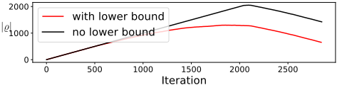
We also test the effect of a simple initial lower bound as proposed in section 3.2 by comparing the cardinality of ϱ during a full run of ExLipBaB with and without an initial lower bound computed on 5 · 106 grid points. On the GroupSort NN from Table 4, the lower bound computation took 5.66 seconds, resulting in a bound of 1.629 and only one fewer subproblem was added to ϱ. On the ReLU NN from Table 3, the lower bound computation took 2.65 seconds with a bound of 1.677. As can be seen in figure 1, this resulted in a drastic reduction of the cardinality of ϱ but the number of iterations needed for an exact ExLipBaB run did not change. The usefulness of a lower bound seems therefore highly dependent on its quality and will most likely only lie in a reduction of required memory. Given its comparatively quick computation time, there is however little downside to using it and especially for low-dimensional inputs a reasonably good coverage of the input space can likely be obtained fairly easily.
| Wine, Network shape [11, 12, 12, 1] | ||||
|---|---|---|---|---|
| Rd0 | ReLU | MaxMin | ||
| estimate | time (s) | estimate | time (s) | |
| Layerwise | 5.86 | 0.000 | 3.78 | 0.000 |
| LipSDP (*) | 1.84 | 26.65 | 2.87 | 0.014 |
| LipSDP (**) | 1.30 | 4.257 | - | - |
| SymProp | 4.78 | 0.015 | 11.09 | 0.013 |
| ExLipBaB | 1.74 | 36.65 | 2.79 | 2.444 |
4.4 Influence of Input Space Size
Unlike the layerwise and LipSDP estimators, our method is not just able to compute the global Lipschitz constant L(f,Rd0 ), but also local constants L(f,Ω) for Ω ⊊ Rd0 . Since generally only a subset of linear regions of f intersects Ω, this can drastically reduce computational cost. Also, local robustness guarantees can potentially be more helpful (tighter) than global ones. We illustrate the aforementioned implications of the size of Ω in Table 6.B for the GroupSort NN from Table 4 and show in Table 6.A the increasing computational cost for an increasing network size. The latter is also further discussed in the supplement.
5 Conclusion
The ExLipBaB algorithm we discussed can compute the exact Lipschitz constant for general continuous piecewise linear NNs. This generalization is of special importance in the field of Lipschitz-constrained NNs in which the ReLU function, which most existing methods are tailored towards, has been shown to have theoretical limitations.
Our generalization also allows a relatively straightforward extension to convolutional and residual NNs in future research. The importance of Lipschitz constant estimation for convolutional neural networks (CNNs) specifically, even for small ones, has been a topic of study in recent years, often in the context of adversarial robustness. In the context of residual NNs, Lipschitz constant estimation is often performed in the method of Residual Normalizing Flows. Such Flows need to keep a balance in their allowed Lipschitz constant to be both invertible and expressive. Both fields would benefit from tighter Lipschitz bounds. However, future research would likely have to leverage the specific structure and sparsity of such NNs, as Branch-and-Bound methods would likely not scale to any but the smallest networks otherwise. Still, our algorithm lends itself naturally to parallelization. In combination with reduced RAM requirements through tighter lower bounds, this could allow computations for more complex NNs and larger input regions.
| Wine, Network shape [11, 24, 24, 1] | ||||
|---|---|---|---|---|
| Rd0 | ReLU | MaxMin | ||
| estimate | time (s) | estimate | time (s) | |
| Layerwise | 5.86 | 0.000 | 6.10 | 0.002 |
| LipSDP | 1.19 | 4.630 | 4.70 | 0.012 |
| SymProp | 4.78 | 0.016 | 25.3 | 0.040 |
| ExLipBaB | 2.62 | (*) | 4.23 | 377.3 |
| Bike sharing, Network shape [13, 20, 16, 8, 3] | ||||
|---|---|---|---|---|
| Rd0 | ReLU | MaxMin | ||
| estimate | time (s) | estimate | time (s) | |
| Layerwise | 30848 | 0.000 | 13145 | 0.000 |
| LipSDP | 5895(*) | 5.041 | 9946 | 0.018 |
| SymProp | 20846 | 0.043 | 58484 | 0.038 |
| ExLipBaB | 10802 | 39283 | - | (**) |
| (A) L(f), f = [13, h1, h2, h3, 1] (ReLU) on [0, 0.1]13 | ||||
| hj | 20, 16, 8 | 32, 32, 32 | 48, 48, 48 | 64, 64, 64 |
| time | 7.42s | 48.1s | 2321s | 6177s |
| L(f ) | 3440 | 4605 | 47.84 | 740.3 |
| (B) L(f), f = [13, 20, 16, 8, 3] (GroupSort) on [-i, i]13 | ||||
| i | 0.1 | 0.2 | 0.4 | 1 |
| time | 5.1s | 40.4s | 136s | 365s |
| L(f ) | 3.32 | 3.61 | 4.12 | 4.23 |
Acknowledgements
This work has been funded by the Deutsche Forschungsgemeinschaft (DFG, German Research Foundation) - 459360854 as part of the Research Unit "Lifespan AI: From Longitudinal Data to Lifespan Inference in Health" (DFG FOR 5347), University of Bremen (https://lifespanai.de/).
We also thank the U Bremen Research Alliance (UBRA) for fostering our research into this topic in their AI Toolbox Hackathon.
@inproceedings{ijcai2026p85,
  title     = {ExLipBaB: Exact Lipschitz Constant Computation for Piecewise Linear Neural Networks},
  author    = {Splittgerber, Tom},
  booktitle = {Proceedings of the Thirty-Fifth International Joint Conference on
               Artificial Intelligence, {IJCAI-26}},
  publisher = {International Joint Conferences on Artificial Intelligence Organization},
  editor    = {Diego Calvanese},
  pages     = {753--761},
  year      = {2026},
  month     = {8},
  note      = {Main Track},
  doi       = {10.24963/ijcai.2026/85},
  url       = {https://doi.org/10.24963/ijcai.2026/85},
}
TY - CPAPER TI - ExLipBaB: Exact Lipschitz Constant Computation for Piecewise Linear Neural Networks AU - Splittgerber, Tom T2 - Proceedings of the Thirty-Fifth International Joint Conference on Artificial Intelligence, IJCAI-26 PB - International Joint Conferences on Artificial Intelligence Organization PY - 2026 SP - 753 EP - 761 DO - 10.24963/ijcai.2026/85 UR - https://doi.org/10.24963/ijcai.2026/85 ER -Copied
Machine-readable versions of this paper, for tools and AI agents:





