
Domain-Informed Graph Neural Networks for Climate Factor Forecasting to Support Sustainable Crop Management
Proceedings of the Thirty-Fifth International Joint Conference on Artificial Intelligence. AI and Social Good. Pages 7437-7445.
https://doi.org/10.24963/ijcai.2026/827
Keywords
- Data Mining: Data Mining
- Multidisciplinary Topics and Applications: Multidisciplinary Topics and Applications
- Machine Learning: Machine Learning
Abstract
Forecasting climate factors is critical for anticipating agro-climatic risks and enabling sustainable crop management. However, accurate prediction remains challenging due to complex spatiotemporal variability, heterogeneous seasonal patterns, and intricate interdependencies among climate variables. Inspired by agronomic knowledge, We propose DoIGNN, a Domain-Informed Graph Neural Network that injects a domain-structured graph constraint built from Agro-Climatic Homogeneous Zones (ACHZs). Specifically, we partition stations into agro-climatic zones using long-term climatic statistics and location attributes, and construct a hierarchical ACHZ-guided adjacency. To better capture shared climate dynamics, we introduce a spatiotemporal decomposition module with temporal regularization that factorizes the climate tensor into low-rank global temporal bases and station loadings, yielding a compact station-level global component as auxiliary information for target forecasting. Finally, DoIGNN performs forecasting on both the ACHZ-guided and static-dynamic graphs to learn cross-region dependencies. Experiments on real-world climate datasets demonstrate that DoIGNN consistently improves forecasting accuracy over strong baselines while yielding more interpretable spatial dependency patterns that support climate-informed crop management decisions. Cooperating with Ningbo Natural Resources and Planning Big Data Center, the proposed model has been trained and deployed for local data analysis.
- [Allen et al., 1998] Richard G. Allen, Luis S. Pereira, Dirk Raes, and Martin Smith. Crop evapotranspiration- guidelines for computing crop water requirements-fao irri- gation and drainage paper 56. Fao, Rome, 300(9):D05109, 1998.
- [Bai et al., 2018] Shaojie Bai, J. Zico Kolter, and Vladlen Koltun. An empirical evaluation of generic convolutional and recurrent networks for sequence modeling, April 2018.
- [Carroll and Chang, 1970] J. Douglas Carroll and Jih-Jie Chang. Analysis of individual differences in multidi- mensional scaling via an n-way generalization of "eckart- young" decomposition. Psychometrika, 35(3):283-319, September 1970.
- [Chen et al., 2022] Chengcheng Chen, Qian Zhang, Mahsa H. Kashani, Changhyun Jun, Sayed M. Bateni, Shahab S. Band, Sonam Sandeep Dash, and Kwok-Wing Chau. Forecast of rainfall distribution based on fixed sliding window long short-term memory. Engineering Ap- plications of Computational Fluid Mechanics, December 2022.
- [Das and Ghosh, 2018] Monidipa Das and Soumya K. Ghosh. Data-driven approaches for meteorological time series prediction: A comparative study of the state-of-the- art computational intelligence techniques. Pattern Recog- nition Letters, 105:155-164, April 2018.
- [Fischer et al., 2012] G. Fischer, F. O. Nachtergaele, S. Prieler, E. Teixeira, G. Toth, H. van Velthuizen, L. Verelst, and D. Wiberg. Global Agro-Ecological Zones (GAEZ v3.0)-Model Documentation. IIASA, Laxenburg, Austria and FAO, Rome, Italy., Laxenburg, Austria; Rome, Italy, 2012.
- [Giorgi et al., 2023] Filippo Giorgi, Erika Coppola, Graziano Giuliani, James M. Ciarlo', Emanuela Pichelli, Rita Nogherotto, Francesca Raffaele, Piero Malguzzi, Silvio Davolio, Paolo Stocchi, and Oxana Drofa. The fifth generation regional climate modeling system, regcm5: Description and illustrative examples at parameterized convection and convection-permitting res- olutions. Journal of Geophysical Research: Atmospheres, 128(6):e2022JD038199, 2023.
- [Gong et al., 2024] Yongshun Gong, Tiantian He, Meng Chen, Bin Wang, Liqiang Nie, and Yilong Yin. Spatio- temporal enhanced contrastive and contextual learning for weather forecasting. IEEE Transactions on Knowledge and Data Engineering, 36(8):4260-4274, August 2024.
- [Gupta et al., 2009] Hoshin V. Gupta, Harald Kling, Ko- ray K. Yilmaz, and Guillermo F. Martinez. Decomposi- tion of the mean squared error and nse performance cri- teria: Implications for improving hydrological modelling. Journal of Hydrology, 377(1):80-91, October 2009.
- [Haggag et al., 2021] May Haggag, Ahmad S. Siam, Wael El-Dakhakhni, Paulin Coulibaly, and Elkafi Hassini. A deep learning model for predicting climate-induced disas- ters. Natural Hazards, 107(1):1009-1034, May 2021.
- [Harshman, 1970] R. A. Harshman. Foundations of the parafac procedure: Models and conditions for an 'ex- planatory' multi-modal factor analysis. Technical Report PB197824, California Univ., Los Angeles., 1970.
- [He et al., 2021a] Kaiming He, Xinlei Chen, Saining Xie, Yanghao Li, Piotr Dollár, and Ross Girshick. Masked au- toencoders are scalable vision learners, December 2021.
- [He et al., 2021b] Sijie He, Xinyan Li, Timothy DelSole, Pradeep Ravikumar, and Arindam Banerjee. Sub-seasonal climate forecasting via machine learning: Challenges, analysis, and advances. Proceedings of the AAAI Confer- ence on Artificial Intelligence, 35(1):169-177, May 2021.
- [Humphries et al., 2026] Usa Wannasingha Humphries, Muhammad Waqas, and Shakeel Ahmad. Novel deep learning framework for rainfall forecasting integrating generative adversarial and spatiotemporal graph neural networks. Results in Engineering, 29:108616, March 2026.
- [Jang et al., 2022] Eric Jang, Shixiang Gu, and Ben Poole. Categorical reparameterization with gumbel-softmax. In International Conference on Learning Representations, July 2022.
- [Kimura, 2002] Ryuji Kimura. Numerical weather predic- tion. Journal of Wind Engineering and Industrial Aerody- namics, 90(12):1403-1414, December 2002.
- [Kolda and Bader, 2009] Tamara G. Kolda and Brett W. Bader. Tensor decompositions and applications. SIAM Review, 51(3):455-500, August 2009.
- [Leutbecher and Palmer, 2008] M. Leutbecher and T. N. Palmer. Ensemble forecasting. Journal of Computational Physics, 227(7):3515-3539, March 2008.
- [Li et al., 2025] Menglin Li, Ming Yang, and Yixiao Yu. Short-term regional wind power forecast method based on hierarchical graph neural network and extreme value the- ory. Energy Conversion and Management, 341:120002, October 2025.
- [Meng et al., 2018] Xianyong Meng, Hao Wang, Chunxiang Shi, Yiping Wu, and Xiaonan Ji. Establishment and eval- uation of the china meteorological assimilation driving datasets for the swat model (cmads). Water, 10(11):1555, November 2018.
- [Middleton et al., 1992] Nick Middleton, David Thomas, and UNEP, editors. World Atlas of Desertification. Ed- ward Arnold : UNEP, London ; New York ; Melbourne, Australia ; Auckland, New Zealand, 1992.
- [Nash and Sutcliffe, 1970] J. E. Nash and J. V. Sutcliffe. River flow forecasting through conceptual models part i -a discussion of principles. Journal of Hydrology, 10(3):282-290, April 1970.
- [Nouri and Veysi, 2025] Milad Nouri and Shadman Veysi. Mitigating crop modeling uncertainties through machine learning in drylands. Scientific Reports, 15(1):42663, November 2025.
- [Utku and Akyol, 2025] Anıl Utku and Sinem Akyol. Hy- brid ga-convlstm for data-driven prediction of climate vari- ables: A case study of the most biodiverse cities in in- dia. Neural Computing and Applications, 37(24):19549- 19578, August 2025.
- [Walsh and Lawler, 1981] R. P. D. Walsh and D. M. Lawler. Rainfall seasonality: Description, spatial patterns and change through time. Weather, 36(7):201-208, 1981.
- [Yousaf et al., 2025] Umair Yousaf, Alessio De Rango, Luca Furnari, Donato D'Ambrosio, Alfonso Senatore, and Giuseppe Mendicino. Spatio-temporal graph neural net- works to improve precipitation forecasts from numerical models. Soft Computing, 29(9):4481-4494, May 2025.
- [Zhang et al., 2026] Gangfeng Zhang, Shuo Wang, Jing Xu, Tim R. McVicar, Yun Cheng, Cesar Azorin-Molina, Lorenzo Minola, Nan Wang, Jiang Zhang, and Peijun Shi. A deep learning approach predicts o3 increase and pm2.5 declines under high emission scenario across the northern china urban agglomeration. Urban Climate, 65:102752, February 2026.
- [Zhao et al., 2025] Junfan Zhao, Fan Zhao, and Hang Deng. Evaluation of climate prediction models in yunnan, china: Traditional methods and ai approaches. Scientific Reports, 15(1):43347, December 2025.
References were extracted automatically from the PDF and may contain errors.
Full text extracted automatically from the PDF; figures, tables and equations may differ. The PDF is the version of record.
1 Introduction
Climate factors, such as temperature, precipitation and humidity, are climatic drivers that directly influence crop phenology, soil moisture dynamics, and pest & disease pressures. Therefore, predicting changes in these factors is irreplaceable for efficient crop management and food security planning [Nouri and Veysi, 2025]. However, achieving high-resolution and robust predictions remains challenging because local climatic dynamics are inherently influenced by surrounding regions. Without explicitly considering the spatial dependencies among neighboring areas, predictions often fail to capture propagating weather patterns and regional interactions, especially at large spatial scales. Moreover, climate regimes vary substantially across regions, exhibiting non-uniform feature distributions and heterogeneous temporal patterns, which makes it difficult for a single model to generalize effectively across diverse agro-climatic zones.
Traditional climate forecasting has long relied on numerical weather prediction (NWP) and climate models grounded in atmospheric dynamics [Kimura, 2002; Leutbecher and Palmer, 2008; Zhao et al., 2025; Giorgi et al., 2023]. These methods have achieved strong performance in large-scale weather and climate simulation by explicitly modeling physical processes. However, their effectiveness often depends on complex physical parameterizations, high-quality boundary conditions, and substantial computational resources, which may limit their flexibility for regional, station-level, and application-oriented agro-climatic forecasting.
To complement physics-based approaches, data-driven models have been increasingly explored for meteorological and climate prediction. Classical machine learning methods such as SVMs and random forests have been used to model nonlinear relationships among meteorological variables [Das and Ghosh, 2018; He et al., 2021b]. Deep learning models, including CNNs, RNNs, ConvLSTMs, and recent spatiotemporal architectures, further improve the ability to capture temporal evolution and spatial patterns from historical observations [Haggag et al., 2021; Chen et al., 2022; Gong et al., 2024; Utku and Akyol, 2025]. Despite these advances, many existing methods still rely mainly on statistical correlations and may insufficiently encode domain-specific agro-climatic structure.
Recently, graph neural networks (GNNs) have shown strong potential in climate-related forecasting by representing stations, grids, or regions as nodes and modeling spatial dependencies through graph propagation [Humphries et al., 2026; Yousaf et al., 2025; Zhang et al., 2026; Li et al., 2025]. Such models are particularly suitable for multi-station forecasting because they can capture non-Euclidean spatial interactions beyond regular grid assumptions. Nevertheless, most existing graph-based methods construct spatial graphs from geographical distance, statistical similarity, or learnable adjacency matrices, while the integration of agro-climatic domain knowledge into graph construction remains underexplored.
Compared with NWP and traditional machine learning methods, deep learning methods-especially graph-based models-exhibit improved performance in capturing nonlinear spatiotemporal correlations of univariate data. Nevertheless, the prediction of climate data via deep learning still encounters the following challenges:
- Existing GNN-based methods construct graphs using geographic proximity, statistical similarity, or fully learnable adjacency. Such topologies are often misaligned with agro-climatic regimes.
- Existing models simply encode all components in a single representation, which may cause representation redundancy.
- Many methods capture only one type of dependency (static or dynamic) or yield opaque learned edges without clear agro-climatic meaning.
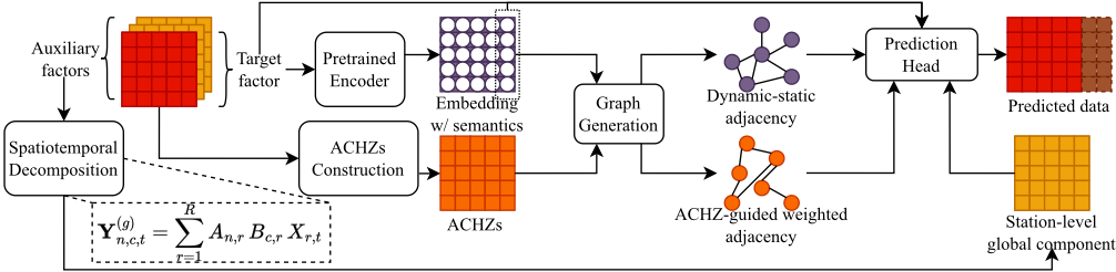
Based on the above challenges, we propose DoIGNN, a Domain-Informed Graph Neural Network, a framework that explicitly integrates agro-climatic domain knowledge into graph-based spatiotemporal modeling. In this approach, climate observation stations are systematically grouped into Agro-Climatic Homogeneous Zones (ACHZs) using long-term meteorological statistics and geospatial attributes. Specifically, intra-zone connections capture localized climatic coherence, while inter-zone links selectively model broader regional interactions and teleconnections. Furthermore, the spatiotemporal decomposition module is introduced to factorizes the multivariate climate tensor into a low-rank set of global temporal bases and station-specific loadings, and then derives a station-level global component that summarizes common spatiotemporal trends for target forecasting. DoIGNN jointly performs prediction over the ACHZ-based and learned graphs, thereby uncovering both cross-variable and cross-regional dependencies. The environmental-resource science domain experts from Ningbo Natural Resources and Planning Big Data Center codeveloped the ACHZ construction by specifying agronomically meaningful indicators and thresholding rules. In addition, they provided domain-relevant criteria for more comprehensive and accurate model evaluation.
The main contributions of this article are as follows.
- DoIGNN partitions stations into ACHZs and constructs a ACHZ-guided hierarchical graph that encourages within-zone edges while selectively allowing cross-zone connections.
- By spatiotemporal decomposition, DoIGNN exploits shared climate dynamics while avoiding excessive reliance on raw auxiliary variables. The temporal regularization further preserves temporal structure, leading to more stable learning and improved robustness.
- DoIGNN performs forecasting on real-word climate datasets validate the effectiveness of our model. Compared with several baseline methods under different prediction horizons, our method demonstrates superior performance.
2 Preliminaries and Problem Statement
2.1 Agro-Climatic Homogeneous Zones (ACHZs)
Agro-Climatic Homogeneous Zones (ACHZs) partition monitoring stations into groups sharing similar long-term agroclimatic regimes (e.g., thermal resources, moisture availability, and rainfall seasonality). Unlike purely data-driven clustering, ACHZs are defined by rule-based agro-climatic indicators computed from multi-decadal daily meteorological records, improving interpretability and aligning the graph structure with agro-ecological principles [Fischer et al., 2012].
Given the annual accumulated Growing Degree Days GDDi, the Aridity Index AIi, and the Seasonality Index SIi, each station i can be assigned to an ACHZ by discretizing these indicators into ordered classes with agronomically meaningful thresholds:
where ϕth, ϕmo, ϕse are rule-based binning functions (e.g., low/medium/high heat, arid-humid regimes, weak-strong seasonality), and ⊕ denotes concatenation into a unique ACHZ identifier. This yields zones that are directly interpretable in terms of agricultural climate constraints, enabling principled spatial regularization in subsequent graph modeling.
2.2 Problem Statement
Consider a multivariate spatiotemporal climate dataset X ∈ RT×N×C , where T denotes the number of time steps (days), N is the number of stations, and C is the number of climate factors. Given a target channel, the goal is to forecast its future values Y ∈ Rf×N over a future horizon of f = 12 days using the historical h = 12 days of all variables.
Formally, for each station n ∈ {1, . . . ,N} and each reference time t satisfying L ≤ t ≤ T -H, we define the input history tensor and prediction target as:
We aim to learn a forecasting function fθ parameterized by θ such that:
where G denotes a set of graphs describing inter-station dependencies.
3 Methods
The DoIGNN architecture mainly consists of ACHZs Construction, graph generation and prediction head module. The schematic diagram of DoIGNN can be seen in Figure 1.
3.1 ACHZs Construction
We construct an ACHZ-guided graph to inject domain knowledge into spatial dependency modeling. Each station is first assigned a zone label using rule-based discretization of longterm agro-climatic indicators, and then a weighted adjacency matrix is derived by combining within-zone consistency with cross-zone similarity.
Let D(y) i denote the set of days in year y at station i. Using daily mean temperature Ti(d) (◦C), daily minimum/maximum temperatures T min i (d), T max i (d) (◦C), daily precipitation Pi(d) (mm), and daily incoming solar radiation Rs,i(d) (MJ m-2 day-1 ), we compute the following longterm descriptors.
Station-Wise Agro-Climatic Descriptors
For station i, we compute a climatological descriptor vector
where Ti is the multi-year mean daily temperature, GDDi(Tb) is the multi-year mean annual GDD with base temperature Tb, FFPi is the mean frost-free period, HDi is the mean number of heat-stress days (e.g., T max ≥ 35◦C).
Thermal Resources via GDD
For a crop-specific base temperature Tb, the annual accumulated GDD is
We use the multi-year climatological mean GDDi = 1 Y ∑y GDD(y) i as a proxy of heat availability, which is widely used to quantify crop development and phenological progress.
Moisture Availability via AI
Following a commonly adopted definition in dryland and agro-environmental studies, we define the aridity index as
where Pi is the multi-year mean annual precipitation (mm year-1 ) and PETi is the multi-year mean annual potential evapotranspiration (mm year-1 ). The AI = P/PET formulation is standard in global aridity characterization [Middleton et al., 1992].
When full meteorological inputs for FAO-56 PenmanMonteith are unavailable, we estimate PET using the Makkink reference evapotranspiration estimator based on solar radiation and pressure-related psychrometric variables, and then aggregate daily ET0 to annual PET [Allen et al., 1998].
Rainfall Seasonality via SI
To characterize intra-annual rainfall concentration, we compute a seasonality index based on monthly precipitation climatology {P i,m}12 m=1 :
where P i and PETi are multi-year mean annual precipitation and potential evapotranspiration, and {Pi,m}12 m=1 is monthly precipitation climatology. SI measures deviation from uniformly distributed rainfall across months and is commonly used to describe rainfall seasonality patterns [Walsh and Lawler, 1981].
3.2 Spatiotemporal Decomposition
Given a 3-D tensor Y ∈ RT×N×C , the decomposition module separates Y into a shared global component and a local residual:
We model Y(g) via a rank-R CANDECOMP/PARAFAC (CP) factorization [Harshman, 1970; Carroll and Chang, 1970; Kolda and Bader, 2009]:
where A ∈ RN×R captures spatial loadings, B ∈ RC×R captures variable loadings, and X ∈ RR×T denotes global temporal factors shared across all stations and variables. Equivalently, Y(g) = ∑Rr=1 ar ◦ br ◦ xr with ◦ being the outer product. The local term is defined as the residual Y(l) = Y - Y(g) .
To encourage temporally consistent dynamics in X, we introduce a one-step predictive regularizer using a Temporal Convolutional Network (TCN) ϕ(·) [Bai et al., 2018]. For a window length w, we penalize deviations from the one-step prediction:
Finally, the factors are estimated by minimizing a regularized reconstruction objective:
where λ, µ > 0 control weight decay and temporal smoothness, respectively. In practice, we solve ((11)) by alternating updates: fixing (B,X) to update A, fixing (A,X) to update B, and fixing (A,B) to update X, while periodically applying the TCN-based temporal step.
For downstream forecasting, we derive a station-wise global representation as auxiliary information by projecting temporal factors through spatial loadings:
To avoid information leakage, the decomposition is fitted using only the training period.
3.3 Pre-trained Encoder
Our encoder follows the masked autoencoder (MAE) paradigm [He et al., 2021a]. Given the input sequences, we perform patch-wise masking and representation learning for each station. For node i, let Xi ∈ RT denote the input sequence, we split it into P non-overlapping patches of length L, where the j-th patch is Xi,j ∈ RL. Then, a high ratio of patches is randomly masked and fed into the corresponding encoder. The encoder is composed of four Transformer blocks to capture temporal patterns, producing patch embeddings Hi j ∈ Rd for local inputs.
Before decoding, masked positions are filled with trainable mask tokens. The decoder contains one Transformer block followed by an MLP head, which reconstructs the j-th patch as ˆXij ∈ RL from Hi j . We optimize the reconstruction error only on masked patches using RMSE:
where M is the number of masked patches, Mm is the corresponding mask matrix, ∥ · ∥F denotes the Frobenius norm, and sum(·) sums all entries of a matrix. After training, the trained encoder can be used to model the overall understanding of the time series, as the autoencoder masks the majority of the input sequence to encourage the learning of high-level semantics.
3.4 Graph Generation
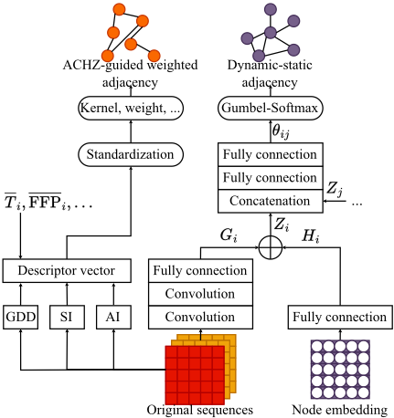
To fully model spatiotemporal dependencies in climate data, DoIGNN constructs (i) a dynamic-static adjacency from node embeddings and raw sequences, and (ii) an ACHZ-guided weighted adjacency. The flowchart is shown in Figure 2.
Dynamic-Static Adjacency
For node i, we extract a static representation from the input sequence Xi via a lightweight CNN-MLP encoder:
where each Conv(·) denotes a convolutional block with convolution, ReLU, and batch normalization, and FC(·) denotes a fully-connected block with ReLU and batch normalization. We then fuse the static feature Gi with the masked embedding Hi to obtain a dynamic-static representation:
We aim to learn a sparse adjacency by modeling edge existence between node pairs. Given Z i and Z j , we compute the Bernoulli logits and probabilities as:
where Θij ∈ R2 denotes unnormalized logits and Θ′ij is the corresponding normalized Bernoulli distribution. To enable end-to-end optimization with discrete sampling, we employ the Gumbel-Softmax reparameterization [Jang et al., 2022]:
where g ∈ R2 is sampled i.i.d. from Gumbel(0, 1) and τ is the temperature. To regularize the learned structure and control sparsity, we introduce a kNN prior graph Ak and penalize deviations using a cross-entropy term:
where Ak specifies the kNN connectivity.
ACHZ-Guided Weighted Adjacency
Let C = [c1, . . . , cN]⊤ be the descriptor matrix. We first standardize each feature dimension:
and define an agro-climatic similarity kernel
where σ controls the kernel bandwidth. The ACHZ-guided weighted adjacency AACHZ is
where λ ∈ (0, 1) down-weights cross-zone connections to emphasize within-zone homogeneity while still allowing weak long-range interactions.
3.5 Prediction Head
We adopt a downstream GNN, an ACHZ-guided Graph WaveNet, to performmulti-step forecasting. To jointly leverage the learned dynamic-static ACHZ-guided weighted adjacency, we treat Ads and AACHZ as undirected graph and obtain forward & backward transitions.
ACHZ-guided Graph WaveNet further employs dilated causal convolutions to capture temporal dependencies. In the fusion layer, we combine the latent representation with the last patch embedding HP to obtain the final prediction:
where Xtarget ∈ RN×T is the target factor. || denotes concatenation, MLP consists of two fully-connected layers with ReLU, and Conv is a 1×1 convolution with ReLU. The output ˆY represents the f-step-ahead forecasts for n nodes.
Finally, we optimize the prediction model using MAE together with the graph regularizer in:
where Y is the ground truth, and λgraph controls the strength of structure regularization. An overview of the full training pipeline is provided in Algorithm 1.
4 Experiments
4.1 Dataset
We use the China Meteorological Assimilation Driving Datasets for the SWAT model-Long time series (CMADS-L V1.0), obtained from the official CMADS portal. 1 CMADS
Algorithm 1: DoIGNN
Input: Past observations: X ∈ RT×N×C . Output: Future forecasts: ˆY ∈ Rf×N . /* Spatiotemporal Decomposition */ 1 for i1 alternating iterations do 2 Fix TCN ϕ(·),A,B update X using Equation (11). 3 Fix TCN ϕ(·),X and update A,B using Equation (11). 4 if mod iteration then 5 Fix A, B, X and update TCN ϕ(·) using Equation (10). 6 end 7 end 8 Obtain station-wise global representation Xaux by Equation (12). /* Pre-trained Encoder */ 9 Split Xinto P patches and mask them with probability p. 10 for i2 epochs do 11 Encode X to obtain H, complement masked positions with trainable patches, and decode to yield ˆX. 12 Update encoder & decoder parameters using Equation (13). 13 end 14 Obtain pretrained node embeddings H. /* Prediction Head */ 15 Compute ACHZ through Equation (4) - (7) 16 Construct ACHZ-guided weighted adjacency AACHZ by Equation (19) - (21). 17 for i3 epochs do 18 Generate dynamic-static adjacency Ads by Equation (14)-(18). /* Prediction module */ 19 Compute transition matrices and perform dilated causal convolutions by Equation (22) to obtain Hgw. 20 Fuse HP and Hgw via (22) to produce ˆY. 21 Update prediction head parameters using (23). 22 endis a meteorological forcing dataset designed for hydrological and agro-environmental applications, produced by assimilating multi-source observations and numerical background fields [Meng et al., 2018]. CMADS V1.0 provides daily meteorological fields over East Asia (approximately 0◦ - 65◦N, 60◦ -160◦E) at 1/3◦ spatial resolution, organized as a 195×300 grid. Climate factors includes: surface atmospheric pressure p (hPa), daily mean temperature ¯ T (◦C), daily maximum/minimum temperatures T max , T min (◦C), 24-hour accumulated precipitation P (mm), relative humidity RH (%), solar radiation Rs (MJm-2 ), specific humidity q (gkg-1 ), and wind speed u (m s-1 ).
In this study, the forecasting target is the daily mean temperature, solar radiation and specific humidity. We subsample N = 130 stations on a regular grid by selecting one site every 15 latitude indices and one site every 30 longitude indices, yielding a 13 × 10 station set.
| Methods | Horizon 3 | Horizon 6 | Horizon 12 | |||||||||
|---|---|---|---|---|---|---|---|---|---|---|---|---|
| MAE | RMSE | NSE | KGE | MAE | RMSE | NSE | KGE | MAE | RMSE | NSE | KGE | |
| AGCRN | 4.5517 | 6.5774 | 0.8542 | 0.8152 | 4.4600 | 6.2099 | 0.8701 | 0.8285 | 4.7601 | 6.5818 | 0.8540 | 0.8152 |
| Crossformer | 3.7753 | 5.0153 | 0.9152 | 0.8641 | 4.1669 | 5.4702 | 0.8992 | 0.8219 | 4.5749 | 5.9810 | 0.8794 | 0.7998 |
| DCRNN | 3.4406 | 4.6053 | 0.9285 | 0.8777 | 3.8580 | 5.1542 | 0.9105 | 0.8665 | 4.2656 | 5.6267 | 0.8933 | 0.8352 |
| GWNet | 3.6785 | 5.0882 | 0.7382 | 0.3256 | 4.1683 | 5.6851 | 0.6733 | 0.3401 | 4.8886 | 6.5952 | 0.5601 | 0.3625 |
| Average MTGNN | 4.3886 | 5.7360 | 0.8891 | 0.7832 | 5.0663 | 6.7010 | 0.8487 | 0.7458 | 6.0572 | 8.0127 | 0.7836 | 0.6836 |
| Temperature STAEformer | 3.1057 | 4.2495 | 0.9391 | 0.8825 | 3.8038 | 5.0490 | 0.9141 | 0.8265 | 4.8632 | 6.2786 | 0.8671 | 0.7442 |
| StemGNN | 3.8485 | 6.1733 | 0.8715 | 0.8301 | 4.1262 | 6.4820 | 0.8584 | 0.8134 | 4.4708 | 6.8545 | 0.8416 | 0.8061 |
| WaveNet | 2.8077 | 4.3968 | 0.2832 | -1.2076 | 3.0342 | 4.7023 | 0.1805 | -1.1916 | 3.4245 | 5.2627 | -0.0270 | -1.1595 |
| DoIGNN | 2.8893 | 4.1478 | 0.9420 | 0.9085 | 3.4268 | 4.8750 | 0.9199 | 0.8829 | 3.9589 | 5.5587 | 0.8958 | 0.8660 |
| AGCRN | 3.5236 | 4.5878 | 0.6971 | 0.7941 | 3.6210 | 4.7080 | 0.6812 | 0.7865 | 3.8030 | 4.9276 | 0.6512 | 0.7668 |
| Crossformer | 3.4260 | 4.5561 | 0.7022 | 0.8246 | 3.4260 | 4.5561 | 0.7022 | 0.8246 | 3.7127 | 4.8695 | 0.6604 | 0.8046 |
| DCRNN | 3.1305 | 4.3004 | 0.7338 | 0.8165 | 3.3518 | 4.5150 | 0.7066 | 0.7935 | 3.7899 | 4.9960 | 0.6411 | 0.7579 |
| GWNet | 3.3451 | 4.4530 | 0.1437 | 0.5076 | 3.3861 | 4.5145 | 0.1203 | 0.5166 | 3.6021 | 4.7356 | 0.0326 | 0.5372 |
| Solar MTGNN | 3.6169 | 4.7857 | 0.6703 | 0.7309 | 3.6169 | 4.7857 | 0.6703 | 0.7309 | 3.9756 | 5.1814 | 0.6141 | 0.6952 |
| Radiation STAEformer | 3.8173 | 5.1648 | 0.6163 | 0.7530 | 4.2601 | 5.8060 | 0.5156 | 0.7079 | 4.2289 | 5.5980 | 0.5500 | 0.7045 |
| StemGNN | 3.3799 | 4.4714 | 0.7123 | 0.7719 | 3.4673 | 4.5763 | 0.6988 | 0.7587 | 3.6776 | 4.8136 | 0.6670 | 0.7381 |
| WaveNet | 3.6020 | 4.8193 | -2.6656 | -0.7193 | 3.7347 | 4.9346 | -2.8409 | -0.6890 | 4.0419 | 5.2053 | -3.2687 | -0.6155 |
| DoIGNN | 3.1399 | 4.3061 | 0.7329 | 0.8131 | 3.2864 | 4.4670 | 0.7127 | 0.7996 | 3.4872 | 4.6463 | 0.6895 | 0.7704 |
| AGCRN | 1.7444 | 2.4009 | 0.8956 | 0.8572 | 1.5971 | 2.1652 | 0.9151 | 0.9036 | 1.6919 | 2.2957 | 0.9046 | 0.8967 |
| Crossformer | 1.6095 | 2.2173 | 0.9110 | 0.8447 | 1.6197 | 2.2797 | 0.9059 | 0.8650 | 1.7733 | 2.4671 | 0.8898 | 0.8393 |
| DCRNN | 1.0926 | 1.5689 | 0.9554 | 0.9469 | 1.2713 | 1.8416 | 0.9386 | 0.9333 | 1.5280 | 2.1906 | 0.9131 | 0.9197 |
| GWNet | 1.6941 | 2.3124 | 0.7096 | 0.3025 | 1.7326 | 2.3770 | 0.6931 | 0.3098 | 1.8507 | 2.5165 | 0.6561 | 0.3169 |
| Specific MTGNN | 2.1349 | 2.8370 | 0.8543 | 0.7399 | 2.3742 | 3.1812 | 0.8168 | 0.7109 | 2.6914 | 3.6306 | 0.7614 | 0.6746 |
| Humidity STAEformer | 1.1062 | 1.5340 | 0.9574 | 0.9583 | 1.2270 | 1.6899 | 0.9483 | 0.9431 | 1.5017 | 1.9961 | 0.9279 | 0.9074 |
| StemGNN | 1.6801 | 2.4713 | 0.8894 | 0.9276 | 1.7825 | 2.5622 | 0.8812 | 0.9336 | 1.8495 | 2.6814 | 0.8698 | 0.9177 |
| WaveNet | 1.1926 | 1.7617 | 0.3819 | -1.2225 | 1.2698 | 1.8571 | 0.3132 | -1.2123 | 1.4167 | 2.0427 | 0.1691 | -1.1907 |
| DoIGNN | 1.0638 | 1.5019 | 0.9592 | 0.9699 | 1.2256 | 1.6847 | 0.9486 | 0.9446 | 1.3746 | 1.8875 | 0.9355 | 0.9358 |
4.2 Evaluation Criteria and Experiment Settings
Beyond point-wise error metrics, we adopt two metrics that are widely used to assess model performance in environmental science and meteorology: Nash-Sutcliffe Efficiency (NSE) [Nash and Sutcliffe, 1970] and the Kling-Gupta Efficiency (KGE) [Gupta et al., 2009].
Let yt(i) and ˆ yt(i) denote the observed and predicted values at station i and time index t over an evaluation window T , and let ¯ y(i) = 1 |T | ∑t∈T yt(i) be the sample mean. The NSE is defined as
NSE quantifies the relative improvement over a mean-value baseline [Nash and Sutcliffe, 1970].
To provide a more diagnostic assessment that disentangles error sources, we further report KGE, which jointly evaluates linear association, bias, and variability [Gupta et al., 2009]:
where r(i) is the Pearson correlation between {yt(i)} and {ˆ yt(i)}, β(i) = µˆ y(i)/µy(i) measures the mean bias ratio, and γ(i) = σˆ y(i)/σy(i) measures the variability ratio, with
µ(·) and σ(·) denoting the sample mean and standard deviation over T . Similar to NSE, values closer to 1 imply better overall agreement [Gupta et al., 2009].
In spatiotemporal decomposition, the learning rate is 0.0005. The temporal regularization parameter λGLD is 0.1. TCN ϕ(·),A,B, X are optimized in 50 iterations and alternate training fashion for every 5 iterations. In embedding module, mask probability p is set as 75%. Embedding and prediction module are both trained for i2 = i3 = 100 times. The learning rate for embedding is 0.0005 without decay, and for prediction is 0.005 with decay. The softmax temperature parameter τ is 0.5. Finally, The graph regularization parameter λgraph is 0.1. Details for ACHZs can be seen in Table 3. Relevant code is available at the project repository.
4.3 Forecasting Results
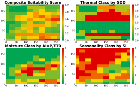
Figure 3 visualizes the constructed ACHZs, which provide an interpretable partition of stations with similar long-term agroclimatic regimes. Table 1 reports the macro-averaged multihorizon forecasting results over all stations, where the best scores are highlighted in bold. Overall, DoIGNN achieved the most consistent performance across horizons and variables, especially on skill-oriented metrics (NSE and KGE), indicating improved predictive reliability beyond point-wise errors.
| Methods | Horizon 3 | Horizon 6 | Horizon 12 | |||||||||
|---|---|---|---|---|---|---|---|---|---|---|---|---|
| MAE | RMSE | NSE | KGE | MAE | RMSE | NSE | KGE | MAE | RMSE | NSE | KGE | |
| DoIGNN w/o AACHZ | 3.3719 | 4.5856 | 0.9291 | 0.8848 | 3.8006 | 5.1667 | 0.9101 | 0.8555 | 4.1501 | 5.5278 | 0.8970 | 0.8406 |
| DoIGNN w/o STD | 3.8264 | 5.1587 | 0.9103 | 0.8772 | 4.4102 | 5.8590 | 0.8843 | 0.8321 | 4.5579 | 6.0073 | 0.8783 | 0.8213 |
| DoIGNNw/o STD, AACHZ | 2.8077 | 4.3968 | 0.2832 | -1.2076 | 3.0342 | 4.7023 | 0.1805 | -1.1916 | 3.4245 | 5.2627 | -0.0270 | -1.1595 |
| DoIGNN | 2.8893 | 4.1478 | 0.9420 | 0.9085 | 3.4268 | 4.8750 | 0.9199 | 0.8829 | 3.9589 | 5.5587 | 0.8958 | 0.8660 |
| Axis | Indicator (unit) | Discretization rule (ordered bins) |
|---|---|---|
| Thermal Moisture Seasonality | GDDi(Tb) (◦C·day/year), Tb = 10◦C AIi = Pi/PETi (-) SIi (-) | [0, 1000), [1000, 2000), [2000, 3000), [3000,∞) [0, 0.2), [0.2, 0.5), [0.5, 0.65), [0.65, 1.0), [1.0, ∞) [0, 0.2), [0.2, 0.4), [0.4, 0.6), [0.6, 0.8), [0.8, ∞) |
Specifically, in average temperature dataset, DoIGNN attains the best overall skill for temperature forecasting, yielding the highest NSE and KGE at all horizons. Notably, some baselines like WaveNet can obtain relatively small MAE but exhibit substantially degraded NSE and KGE. This discrepancy suggests that those models without graph information may fit the central tendency while failing to reproduce the temporal variability and correlation structure. GWNet, on the other hand, markedly improved prediction errors by integrating GCN rather than TCN for spatial relationship analysis. This underscored the significance of graph relationships from domain knowledge in augmenting predictive performance of climate factor.
Finally, Table 2 demonstrates the ablation study results. Removing the ACHZ-guided adjacency (AACHZ ) causes a clear degradation in NSE/KGE, indicating that domainconsistent spatial constraints are critical for preserving forecast skill and preventing spurious cross-regime message passing. Removing the spatiotemporal decomposition (STD) further deteriorates performance, confirming that explicitly extracting global shared dynamics improves stability and generalization. When both STD and AACHZ are removed, the model collapses to the WaveNet-style backbone and exhibits the same behavior as the corresponding baseline, demonstrating that the performance gains of DoIGNN primarily come from the proposed domain-informed graph prior and the global-local decomposition rather than architectural scaling alone.
5 Discussion
The proposed forecasting model can be deployed as a decision-support component for crop management. Given multi-station predictions of climate factors over the forthcoming horizon, the system can derive risk-aware indicators at the zone and field scales such as heat & cold stress likelihood, rainfall deficit & excess, and humidity-driven disease favorability. These indicators enable practitioners to (i) schedule irrigation and drainage by anticipating short-term water stress, (ii) adjust sowing, fertilization, and harvest windows to avoid adverse temperature/rainfall regimes, and (iii) trigger early warnings for pest and fungal disease management under highrisk humidity-temperature patterns. By aggregating forecasts within agro-climatic homogeneous zones, the framework also supports coherent regional planning.
6 Conclusion
This paper presented DoIGNN, a domain-informed graph neural network for climate factor forecasting. DoIGNN injects agro-climatic knowledge via an ACHZ-guided adjacency, and further employs a temporally-regularized globallocal spatiotemporal decomposition to obtain compact shared dynamics as auxiliary information. Built upon the ACHZ constraint and a learned dynamic-static dependency, the proposed prediction model jointly captures cross-region and cross-variable interactions. Experiments on CMADS demonstrate consistent improvements over strong baselines across horizons. In the future, we will focus on lightweight and scalable modeling for long-horizon forecasting over large-scale climate archives to reduce computational and storage costs without sacrificing predictive skill.
Ethical Statement
There are no ethical issues.
Acknowledgements
This work is supported by National Key R&D Program of China (Grant No. 2021YFC2101100), National Natural Science Foundation of China (62073288, 12075212), and Zhejiang University NGICS Platform, and their supports are thereby acknowledged.
@inproceedings{ijcai2026p827,
  title     = {Domain-Informed Graph Neural Networks for Climate Factor Forecasting to Support Sustainable Crop Management},
  author    = {Sun, Ziyue and Jiang, Zixin and Xu, Chenkai and Liu, Xinggao},
  booktitle = {Proceedings of the Thirty-Fifth International Joint Conference on
               Artificial Intelligence, {IJCAI-26}},
  publisher = {International Joint Conferences on Artificial Intelligence Organization},
  editor    = {Diego Calvanese},
  pages     = {7437--7445},
  year      = {2026},
  month     = {8},
  note      = {AI and Social Good},
  doi       = {10.24963/ijcai.2026/827},
  url       = {https://doi.org/10.24963/ijcai.2026/827},
}
TY - CPAPER TI - Domain-Informed Graph Neural Networks for Climate Factor Forecasting to Support Sustainable Crop Management AU - Sun, Ziyue AU - Jiang, Zixin AU - Xu, Chenkai AU - Liu, Xinggao T2 - Proceedings of the Thirty-Fifth International Joint Conference on Artificial Intelligence, IJCAI-26 PB - International Joint Conferences on Artificial Intelligence Organization PY - 2026 SP - 7437 EP - 7445 DO - 10.24963/ijcai.2026/827 UR - https://doi.org/10.24963/ijcai.2026/827 ER -Copied
Machine-readable versions of this paper, for tools and AI agents:





