
PhyTTA: Physics-Informed Test-Time Adaptation of Foundation Models for Regional Drought Prediction
Proceedings of the Thirty-Fifth International Joint Conference on Artificial Intelligence. AI and Social Good. Pages 7147-7155.
https://doi.org/10.24963/ijcai.2026/795
Keywords
- Multidisciplinary Topics and Applications: Multidisciplinary Topics and Applications
- AI4G: Data Mining
- AI4G: Humans and AI
Abstract
Drought prediction is crucial for disaster mitigation, yet it remains challenging because regional droughts reflect nonlinear interactions among precipitation supply, evaporative demand, and slowly varying land atmosphere states. Although time series foundation models (TSFMs) have shown strong zero shot performance in general forecasting tasks, they can exhibit systematic sensitivity mismatch in the prediction of regional precipitation and temperature anomalies in the Standardized Precipitation Evapotranspiration Index (SPEI). We introduce PhyTTA, a physics informed test time adaptation framework that keeps the TSFM backbone frozen and corrects the predictable part of its one step residual through three components: a dynamic forcing correction, a static tracker of slowly varying background bias, and a conditional confidence gate that applies the correction only in supported regimes. Our analysis shows that, when frozen model residuals contain a component predictable from local forcing changes or slowly varying background bias, correcting this component reduces expected squared error in the population setting. PhyTTA implements this principle through a conservative online ridge EMA correction with regime support gating. Across four foundation backbones on three South Australian locations and TimesFM on three cross regional regions, PhyTTA reduces MSE by up to 19.78%. With the TimesFM backbone it gives consistent 12.3% to 15.1% MSE reductions across the three South Australian locations.
- [Ansari et al., 2024] Abdul Fatir Ansari, Lorenzo Stella, Caner Turkmen, et al. Chronos: Learning the language of time series. Transactions on Machine Learning Research, 2024.
- [Bai et al., 2018] Shaojie Bai, J. Zico Kolter, and Vladlen Koltun. An empirical evaluation of generic convolutional and recurrent networks for sequence modeling. arXiv preprint arXiv:1803.01271, 2018.
- [Beguería et al., 2014] Santiago Beguería, Sergio M. Vicente-Serrano, Fergus Reig, and Borja Latorre. Stan- dardized precipitation evapotranspiration index (SPEI) revisited: Parameter fitting, evapotranspiration models, tools, datasets and drought monitoring. International Journal of Climatology, 34(10):3001-3023, 2014.
- [Belgiu and Drȃguţ, 2016] Mariana Belgiu and Lucian Drȃguţ. Random forest in remote sensing: A review of applications and future directions. ISPRS Journal of Photogrammetry and Remote Sensing, 114:24-31, 2016.
- [Box et al., 2015] George E. P. Box, Gwilym M. Jenkins, Gregory C. Reinsel, and Greta M. Ljung. Time Series Analysis: Forecasting and Control. Wiley, Hoboken, NJ, 5 edition, 2015.
- [Chen et al., 2023] Si-An Chen, Chun-Liang Li, Nate Yoder, et al. TSMixer: An all-MLP architecture for time series forecasting. Transactions on Machine Learning Research, 2023.
- [Chen et al., 2025a] Liangzhi Chen, Philipp Brun, Pascal Buri, et al. Global increase in the occurrence and impact of multiyear droughts. Science, 387(6731):278-284, 2025.
- [Chen et al., 2025b] Ying Chen, Huanping Wu, Nengfu Xie, et al. STAT-LSTM: A multivariate spatiotemporal fea- ture aggregation model for SPEI-based drought prediction. Earth Science Informatics, 18(3):289, 2025.
- [Cho et al., 2014] Kyunghyun Cho, Bart van Merriënboer, Caglar Gulcehre, Dzmitry Bahdanau, Fethi Bougares, Holger Schwenk, and Yoshua Bengio. Learning phrase representations using RNN encoder-decoder for statistical machine translation. In Proceedings of the 2014 Confer- ence on Empirical Methods in Natural Language Process- ing (EMNLP), pages 1724-1734, 2014.
- [Dai, 2011] Aiguo Dai. Drought under global warming: A review. Wiley Interdisciplinary Reviews: Climate Change, 2(1):45-65, 2011.
- [Dai, 2013] Aiguo Dai. Increasing drought under global warming in observations and models. Nature Climate Change, 3(1):52-58, 2013.
- [Das et al., 2024] Abhimanyu Das, Weihao Kong, Rajat Sen, and Yichen Zhou. A decoder-only foundation model for time-series forecasting. In Proceedings of the 41st Inter- national Conference on Machine Learning, pages 10148- 10167, 2024.
- [Eyring et al., 2024] Veronika Eyring, William D. Collins, Pierre Gentine, et al. Pushing the frontiers in climate mod- elling and analysis with machine learning. Nature Climate Change, 14:916-928, 2024. [Google Research, 2025] Google Research. TimesFM-2.5: Time series foundation model (pretrained check- point). https://huggingface.co/google/timesfm-2. 5-200m-pytorch, 2025. Accessed 2026-05-28. Link
- [Hochreiter and Schmidhuber, 1997] Sepp Hochreiter and Jürgen Schmidhuber. Long short-term memory. Neural Computation, 9(8):1735-1780, 1997.
- [Hollmann et al., 2025] Noah Hollmann, Samuel Müller, Lennart Purucker, et al. Accurate predictions on small data with a tabular foundation model. Nature, 637(8045):319- 326, 2025.
- [Hyndman and Athanasopoulos, 2021] Rob J. Hyndman and George Athanasopoulos. Forecasting: Principles and Practice. OTexts, Melbourne, Australia, 3 edition, 2021.
- [Hyndman et al., 2002] Rob J. Hyndman, Anne B. Koehler, Ralph D. Snyder, and Simone Grose. A state space framework for automatic forecasting using exponential smoothing methods. International Journal of Forecasting, 18(3):439-454, 2002.
- [Iglesias-Suarez et al., 2024] Fernando Iglesias-Suarez, Pierre Gentine, Breixo Soliño-Fernandez, et al. Causally- informed deep learning to improve climate models and projections. Journal of Geophysical Research: Atmospheres, 129(4):e2023JD039202, 2024.
- [Kalnay et al., 1996] Eugenia Kalnay, Masao Kanamitsu, Robert E. Kistler, et al. The NCEP/NCAR 40-year re- analysis project. Bulletin of the American Meteorological Society, 77(3):437-471, 1996.
- [Karniadakis et al., 2021] George Em Karniadakis, Ioan- nis G. Kevrekidis, Lu Lu, et al. Physics-informed machine learning. Nature Reviews Physics, 3(6):422-440, 2021.
- [Kim et al., 2022] Taesung Kim, Jinhee Kim, Yunwon Tae, et al. Reversible instance normalization for accurate time- series forecasting against distribution shift. In Proceedings of the International Conference on Learning Representa- tions, 2022.
- [Kim et al., 2025] HyunGi Kim, Siwon Kim, Jisoo Mok, and Sungroh Yoon. Battling the non-stationarity in time se- ries forecasting via test-time adaptation. In Proceedings of the AAAI Conference on Artificial Intelligence, volume 39, pages 17868-17876, 2025.
- [Liu et al., 2024a] Xuebang Liu, Shuying Yu, Zhiwei Yang, et al. The first global multi-timescale daily SPEI dataset from 1982 to 2021. Scientific Data, 11:223, 2024.
- [Liu et al., 2024b] Yong Liu, Tengge Hu, Haoran Zhang, Haixu Wu, Shiyu Wang, Lintao Ma, and Mingsheng Long. iTransformer: Inverted transformers are effective for time series forecasting. In Proceedings of the International Conference on Learning Representations, 2024.
- [Marshall, 2003] Gareth J. Marshall. Trends in the Southern Annular Mode from observations and reanalyses. Journal of Climate, 16(24):4134-4143, 2003.
- [Medeiros et al., 2025] Heitor R. Medeiros, Hossein Sharifi- Noghabi, Gabriel L. Oliveira, and Saghar Irandoust. Accu- rate parameter-efficient test-time adaptation for time series forecasting. In ICML 2025 Workshop on Test-Time Adap- tation: Putting Updates to the Test (PUT), 2025.
- [Nguyen et al., 2023] Tung Nguyen, Johannes Brandstetter, Ashish Kapoor, Jayesh K. Gupta, and Aditya Grover. Cli- maX: A foundation model for weather and climate. In Pro- ceedings of the 40th International Conference on Machine Learning, pages 25904-25938, 2023.
- [Nie et al., 2023] Yuqi Nie, Nam H. Nguyen, Phanwadee Sinthong, and Jayant Kalagnanam. A time series is worth 64 words: Long-term forecasting with transformers. In Proceedings of the International Conference on Learning Representations, 2023.
- [Paszke et al., 2019] Adam Paszke, Sam Gross, Francisco Massa, et al. PyTorch: An imperative style, high- performance deep learning library. In Proceedings of Advances in Neural Information Processing Systems (NeurIPS), volume 32, 2019.
- [Prior Labs, 2025] Prior Labs. tabpfn-time-series: Time- series forecasting with TabPFN. https://pypi.org/project/ tabpfn-time-series/1.0.8/, 2025. Version 1.0.8, accessed 2026-05-28. Link
- [Reichstein et al., 2019] Markus Reichstein, Gustau Camps- Valls, Bjorn Stevens, et al. Deep learning and process un- derstanding for data-driven Earth system science. Nature, 566(7743):195-204, 2019.
- [Runge et al., 2023] Jakob Runge, Andreas Gerhardus, Gherardo Varando, et al. Causal inference for time series. Nature Reviews Earth & Environment, 4:487-505, 2023.
- [Saji et al., 1999] N. H. Saji, B. N. Goswami, P. N. Vinay- achandran, and T. Yamagata. A dipole mode in the tropical Indian ocean. Nature, 401(6751):360-363, 1999.
- [Seabold and Perktold, 2010] Skipper Seabold and Josef Perktold. Statsmodels: Econometric and statistical mod- eling with Python. In Proceedings of the 9th Python in Science Conference, pages 92-96, 2010.
- [Trenberth et al., 2014] Kevin E. Trenberth, Aiguo Dai, Ger- ard van der Schrier, et al. Global warming and changes in drought. Nature Climate Change, 4(1):17-22, 2014.
- [Trenberth, 1984] Kevin E. Trenberth. Signal versus noise in the Southern Oscillation. Monthly Weather Review, 112(2):326-332, 1984.
- [Trenberth, 1997] Kevin E. Trenberth. The definition of El Niño. Bulletin of the American Meteorological Society, 78(12):2771-2777, 1997.
- [Vaswani et al., 2017] Ashish Vaswani, Noam Shazeer, Niki Parmar, et al. Attention is all you need. In Proceed- ings of Advances in Neural Information Processing Sys- tems (NeurIPS), volume 30, pages 5998-6008, 2017.
- [Vicente-Serrano et al., 2010] Sergio M. Vicente-Serrano, Santiago Beguería, and Juan I. López-Moreno. A multiscalar drought index sensitive to global warming: The Standardized Precipitation Evapotranspiration Index. Journal of Climate, 23(7):1696-1718, 2010.
- [Wang et al., 2021] Dequan Wang, Evan Shelhamer, Shaoteng Liu, et al. Tent: Fully test-time adaptation by entropy minimization. In Proceedings of the International Conference on Learning Representations, 2021.
- [Wilson and Cook, 2020] Garrett Wilson and Diane J. Cook. A survey of unsupervised deep domain adaptation. ACM Transactions on Intelligent Systems and Technology, 11(5):1-46, 2020.
- [Woo et al., 2024] Gerald Woo, Chenghao Liu, Akshat Ku- mar, Caiming Xiong, Silvio Savarese, and Doyen Sahoo. Unified training of universal time series forecasting trans- formers. In Proceedings of the 41st International Confer- ence on Machine Learning, pages 53140-53164, 2024.
- [Wu et al., 2021] Haixu Wu, Jiehui Xu, Jianmin Wang, and Mingsheng Long. Autoformer: Decomposition transform- ers with auto-correlation for long-term series forecast- ing. In Proceedings of Advances in Neural Information Processing Systems (NeurIPS), volume 34, pages 22419- 22430, 2021.
- [Wu et al., 2023a] Haixu Wu, Tengge Hu, Yong Liu, et al. Time-series-library. https://github.com/thuml/ Time-Series-Library, 2023. Accessed 2026-05-28. Link
- [Wu et al., 2023b] Haixu Wu, Tengge Hu, Yong Liu, Hang Zhou, Jianmin Wang, and Mingsheng Long. TimesNet: Temporal 2D-variation modeling for general time series analysis. In Proceedings of the International Conference on Learning Representations, 2023.
- [Zeng et al., 2023] Ailing Zeng, Muxi Chen, Lei Zhang, et al. Are transformers effective for time series forecast- ing? In Proceedings of the AAAI Conference on Artificial Intelligence, volume 37, pages 11121-11128, 2023.
- [Zhang and Yan, 2023] Yunhao Zhang and Junchi Yan. Crossformer: Transformer utilizing cross-dimension de- pendency for multivariate time series forecasting. In Proceedings of the International Conference on Learning Representations, 2023.
- [Zhou et al., 2022] Tian Zhou, Ziqing Ma, Xue Wang, et al. FiLM: Frequency improved Legendre memory model for long-term time series forecasting. In Proceedings of Advances in Neural Information Processing Systems (NeurIPS), volume 35, pages 12677-12690, 2022.
References were extracted automatically from the PDF and may contain errors.
Full text extracted automatically from the PDF; figures, tables and equations may differ. The PDF is the version of record.
1 Introduction
Drought is one of the most expensive natural disasters, causing billions of dollars in agricultural losses annually and threatening water security for millions of people [Dai, 2011; Trenberth et al., 2014]. The global land area affected by multiyear droughts has expanded steadily over the past four decades [Chen et al., 2025a]. Accurate regional drought prediction is therefore important for water resource management, agricultural planning, and early warning systems. The Standardized Precipitation Evapotranspiration Index (SPEI) is widely used for this purpose because it combines precipitation deficits and temperature induced evaporative demand in a single water balance index [Vicente-Serrano et al., 2010; Beguería et al., 2014].
Traditional drought forecasting has relied on statistical models such as Autoregressive Integrated Moving Average (ARIMA) and Seasonal ARIMA (SARIMA), but these models typically assume stationarity and struggle to represent nonlinear climate dynamics [Box et al., 2015; Hyndman and Athanasopoulos, 2021]. Traditional machine learning models reduce some of these restrictions, but they often require extensive feature engineering [Belgiu and Dr˘agu¸t, 2016]. Deep architectures such as LSTMs [Hochreiter and Schmidhuber, 1997] and Transformers [Vaswani et al., 2017] can learn latent representations directly from data and model long term dependencies, including direct applications to SPEI based drought forecasting [Chen et al., 2025b]. However, training such models from scratch is difficult when high quality regional drought records are limited. This data scarcity constraint motivates the use of pretrained forecasting models rather than purely region specific training.
Recent advances in foundation models appear well suited to this challenge. Time series foundation models (TSFMs) such as TimesFM [Das et al., 2024], Chronos [Ansari et al., 2024], and Moirai [Woo et al., 2024] have demonstrated strong zero shot forecasting across regions. Trained on large heterogeneous corpora, they provide a practical starting point for climate tasks where local data are scarce [Nguyen et al., 2023]. However, when applied to regional drought prediction they can exhibit systematic biases: broad heterogeneous pre training does not necessarily encode localized climate sensitivities driven by region specific soil moisture, vegetation, and evaporative demand processes [Reichstein et al., 2019; Dai, 2011].
The immediate question is therefore not whether to retrain the foundation model, but whether its regional residuals contain a predictable component that can be corrected safely at inference time. Existing time series Test Time Adaptation (TTA) methods such as TAFAS [Kim et al., 2025] and the concurrent PETSA [Medeiros et al., 2025] adapt calibration layers or low rank modules during inference, but gradient updates on small noisy regional streams may degrade performance under distribution shift [Wang et al., 2021; Wilson and Cook, 2020]. We use TAFAS as the representative gradient based benchmark. RevIN [Kim et al., 2022] performs statistical normalization but does not distinguish forcing linked residuals from random weather variability.
In climate science, regional forecasting errors can be addressed better with physical and process understanding, not by statistical alignment alone [Eyring et al., 2024; Reichstein et al., 2019]. Physics informed machine learning work argues that physical constraints and causally informed features can improve robustness and generalization [Karniadakis et al., 2021; Eyring et al., 2024; Runge et al., 2023; Iglesias-Suarez et al., 2024]. We put this perspective into practice by using physical forcing variables, observed climate drivers of the SPEI water balance such as precipitation, maximum temperature, humidity, and air temperature, as predictors of the foundation model residual.
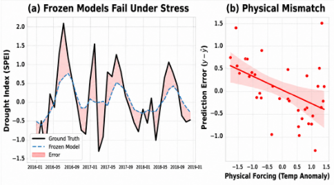
This residual correction view appears empirically in regional SPEI forecasting. Figure 1(a) shows that the frozen TimesFM model produces conservative predictions and dampens extreme SPEI fluctuations during drought events. Figure 1(b) plots TimesFM residuals against the within event temperature anomaly, defined as the month to month change in maximum temperature in the same episode. In hotter than normal months, the model tends to underpredict drought severity, so part of its residual moves with the anomaly and is correctable. Table 4 reports the corresponding correlations between residuals and physical forcing.
Based on the example in Figure 1, we formulate test time adaptation of frozen foundation models for regional drought prediction as conditional residual modeling. If a TSFM has a regional sensitivity mismatch in its SPEI prediction under precipitation or temperature changes, then part of its one step residual is physically informed and predictable. Residual variations not explained by recent target history or physical forcing are treated as stochastic and should not be amplified. PhyTTA therefore corrects the frozen forecast only when the current feature regime is close to recently observed regimes. It realizes this through three components: a dynamic forcing corrector, a static background bias tracker, and a conditional confidence gate.
In summary, our contributions are as follows:
- We formalize test time adaptation of frozen foundation models for regional drought prediction as physics guided conditional residual correction.
- We introduce the PhyTTA framework, which corrects the predictable part of the residual through three complementary components.
- We provide a formal analysis of the framework and show up to 19.78% MSE reduction in evaluations of four TSFM backbones on South Australian locations and the TimesFM backbone on cross regional tests.
2 Problem Setting
Let yt ∈ R be the target SPEI value and ct ∈ Rd be the climate covariate vector at time t. We define the input Xt as the concatenation of historical targets and covariates over a lookback window L:
We focus on one step ahead forecasting (H = 1) with a frozen TSFM fθ :
where θ denotes frozen backbone parameters and the superscript (0) denotes the base uncorrected forecast. Our goal is to produce a corrected forecast ˆ yt+1 without updating θ. The state vector St in Section 3.2 is a compact target history summary derived fromXt and used only by the residual corrector.
The quantity PhyTTA corrects is the one step residual rt+1 = yt+1 - ˆ y(0) t+1 , and E[·] denotes expectation. At test time, yt+1 is never used before predicting ˆ yt+1. After the observation becomes available, it is used only to update the residual buffer for future forecasts. Thus, PhyTTA follows a rolling delayed feedback protocol, in which each label arrives one step after its forecast, rather than label free test time adaptation [Wang et al., 2021; Kim et al., 2025].
3 Method
3.1 The PhyTTA Framework
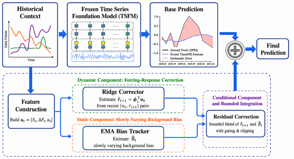
As shown in Figure 2, PhyTTA keeps the foundation model frozen and corrects its forecast along two paths. The top path maps the historical context to the base forecast ˆ y(0) t+1 . The bottom path forms two correction signals: a dynamic forcing residual ˆ rt+1 from a ridge corrector (Section 3.2) and a static slowly varying bias ˆBt from an exponential moving average tracker (Section 3.3). A conditional confidence gate keeps the correction only in supported regimes, and a bounded blend merges the two signals into the adjustment added to ˆ y(0) t+1 (Section 3.4).
3.2 Dynamic Component: Forcing Correction
The dynamic component in Figure 2 corrects the part of the residual correlated with recent forcing changes. It is a single linear ridge corrector over
built from the drought state St, current forcing change ∆Ft, and latest value at = yt. The state and forcing blocks play complementary roles:
- The system state (St) captures the system's internal inertia and "memory." Since drought is an autoregressive process, the magnitude of the prediction error is often state dependent.
- The physical forcing (∆Ft) represents the external drivers (precipitation and temperature changes) that drive the system's evolution.
System State Features (St). We capture drought inertia using target history statistics. St contains full context descriptors over L and short window descriptors over w = 16 months, a short window spanning slightly more than one annual cycle:
where µ and σ are the rolling mean and standard deviation over the window, applied to the target y and to its one step change ∆yi = yi - yi-1.
Physical Forcing Features (∆Ft). From ct, we extract precipitation and temperature, the two primary physical drivers of SPEI, and two auxiliary atmospheric covariates used in the implementation:
where Pt denotes monthly precipitation, ∆Pt = Pt - Pt-1, ∆T max t = T max t -T max t-1 , ∆Qt = Qt -Qt-1, and ∆T air t = T air t - T air t-1 . Here T max t denotes the monthly value derived from daily maximum near surface temperature, Qt denotes monthly specific humidity, and T air t denotes monthly mean near surface air temperature, all taken from NCEP-NCAR Reanalysis 1 [Kalnay et al., 1996]. Because ∆Ft is a one step difference, it lets the corrector respond to immediate forcing changes.
Ridge corrector. The dynamic correction is the ridge prediction ˆ rt+1 = ϕ⊤t ut, where ϕt is the ridge weight vector. PhyTTA keeps a buffer of the most recent N feature residual pairs,
updated only after each forecast is made, using rt+1 = yt+1ˆ y(0) t+1 . We fit ϕt by ridge regression on the pairs (ui, ri+1) with penalty γ∥ϕ∥22 , which has a closed form solution. We use N = 100, warm up Nmin = 30, and γ = 0.5; before warm up, PhyTTA returns the base forecast. The short buffer lets ϕt update with recent conditions, and Eq. (9) combines this fast estimate with the slow background estimate.
3.3 Static Component: Slowly Varying Background Bias
The static component, the lower branch in Figure 2, tracks the slow bias signal ˆBt. The dynamic corrector targets residual variations that move with recent state and forcing changes, but it cannot reliably remove a persistent offset between the frozen forecast and the observed target. Let Bt denote the latent low frequency component of the frozen model residual, representing a slowly varying regional offset between the base forecast and the observed target. Since Bt is not directly observed, we estimate its running value from past residuals using a separate slow channel, an exponential moving average (EMA):
Here ˆBt is the exponential moving average estimate of the latent low frequency bias Bt, and αB = 0.3.
The EMA is a low pass filter: it smooths fast residual fluctuations and tracks a slowly moving baseline. Since each update retains a (1-αB) share of the previous estimate, isolated residual outliers have limited influence. Thus, "static" means slow relative to the fast ridge corrector, not time invariant. This slow offset differs from two other slow quantities in the method: the state memory inside St, which is only an input to the dynamic corrector, and the temporal correlation of the forcing changes themselves.
3.4 Conditional Component and Bounded Integration
The dynamic and static estimates are candidate correction signals; neither is always safe to apply. PhyTTA therefore uses a support gate for unfamiliar regimes and a bounded blend to cap accepted corrections.
Confidence gate. We measure regime support by the nearest neighbor distance to the residual buffer in standardized feature space:
Here qt ∈ (0, 1] is a support score, with larger values meaning closer buffered support. The score is used only after |Wt| ≥ Nmin. If qt > τ, PhyTTA applies the residual correction; otherwise it returns the frozen forecast ˆ y(0) t+1 . We set τ = 0.10 after checking {0.05, 0.10, 0.15} on validation; no test set tuning is used. Feature z scores are fixed from the training and warm up portion.
Bounded blend. When themain gate is open, the final forecast combines ˆ rt+1 and ˆBt, then clips the result. The static estimate is included only when the stricter bias gate qt > τB is satisfied. When the main gate is closed, the correction is zero:
Here clip(x, a, b) = min{max{x, a}, b} and I(·) equals 1 when its condition is true and 0 otherwise. Constants are held fixed across backbones and regions. The step size λ = 0.8 < 1 is conservative, and ω = 0.3 < 0.5 keeps the fast forcing term dominant over the slowly varying bias. The clips are safety rails on the standardized SPEI scale: cy = 3.5 avoids truncating plausible forecasts, while cr = 1.5 caps any single residual correction. The bias gate τB = 0.60 > τ controls only whether the EMA bias term enters the blend.
Online update order. The delayed feedback protocol in Section 2 is implemented as follows. At each step t, PhyTTA first computes the frozen forecast ˆ y(0) t+1 = fθ(Xt) from the available history and constructs ut. If |Wt| < Nmin, it returns the frozen forecast. Otherwise, it fits the ridge corrector on Wt, computes ˆ rt+1, qt, ¯ gt, and the corrected forecast ˆ yt+1 by Eq. (9). In both cases, yt+1 is used only after it becomes available: the method then computes rt+1 = yt+1 - ˆ y(0) t+1 , updates Wt+1, and updates the EMA estimate ˆBt+1. Thus, each newly observed label affects only later forecasts.
4 Theoretical Analysis
Our analysis is conditional on the existence of a predictable component in the frozen model residual. It does not claim that every finite buffer online update improves every test point. Instead, it shows that if the residual contains a component predictable from the features already used by PhyTTA, then correcting this component reduces expected squared error.
4.1 Why Residual Correction Helps
Recall that rt+1 = yt+1 - ˆ y(0) t+1 is the one step residual of the frozen backbone and ut = [St,∆Ft, at] is the feature vector used by the residual corrector. We first analyze the population target estimated by the online ridge corrector.
Proposition 1 (Predictable residual correction reduces error). Let ˆ rt+1 = ϕ⊤t ut be the best penalized linear fit of rt+1 from ut, corresponding to the population version of the ridge corrector in Section 3.2. Then
The inequality is strict whenever rt+1 contains a nonzero feature correlated component that is not fully shrunk to zero by the ridge penalty.
Proof. The zero correction is always feasible: setting ϕt = 0 gives ˆ rt+1 = 0, which recovers the frozen forecast. Since ˆ rt+1 is the best penalized linear fit, its penalized error cannot exceed that of zero correction:
Because the ridge penalty is nonnegative, the unpenalized squared error after correction is also no larger than E[r2 t+1 ]. Strict reduction occurs when a nonzero predictable residual component is fitted rather than suppressed.
This result explains the target of the dynamic ridge component, not an unconditional guarantee for every finite buffer estimate. In practice, the estimate can be noisy when the current feature regime is poorly supported by recent history. This motivates the confidence gate, shrinkage factor λ < 1, and clipping in Eq. (9): the correction is applied only when qt > τ and its magnitude is bounded.
The EMA term targets a different predictable component: a slowly varying residual offset. It is not treated as the intercept of the ridge proof. Instead, Eq. (7) estimates a low frequency bias ˆBt from past residuals only. If recent residuals share a persistent sign, ˆBt is aligned with the next residual and can reduce squared error by the same principle. The stricter gate τB > τ reflects that this bias term shifts the forecast baseline and should be used only in strongly supported regimes.
4.2 When the Premise Holds for SPEI
The above argument is useful only when the frozen model residual is predictable from ut. This premise is natural in regional SPEI forecasting.
Corollary 1 (SPEI residual predictability). Suppose that the one step residual after subtracting the frozen backbone forecast, rt+1 = yt+1 - ˆ y(0) t+1 , contains a nonzero component that is linearly predictable from the forecast time features ut = [St,∆Ft, at]. In regional SPEI forecasting, such a component can arise from a forcing mismatch with respect to precipitation change, temperature change, or recent drought state. Then the population residual correction in Proposition 1 reduces the expected squared error, with strict reduction when this predictable component is not fully shrunk to zero by the ridge penalty.
SPEI reflects the climatic water balance: precipitation contributes to water supply, while temperature affects evaporative demand [Vicente-Serrano et al., 2010; Beguería et al., 2014]. A frozen foundation model trained on heterogeneous time series may learn a useful average forecasting rule but still misrepresent local forcing sensitivity. When this happens, the missed regional response remains in the one step residual and can move with ∆Ft, St, or the anchor at = yt.
The sign of this association between residuals and forcing is not interpreted as the physical sign of the SPEI response itself. It reflects whether the frozen model underestimates or overestimates the local forcing response. Our claim is predictive: if the residual is associated with observable forecast time features, then a residual corrector can use that association.
Monthly drought dynamics further support this premise because SPEI has persistence through precipitation deficits, evaporative demand, soil moisture memory, and large scale climate modes [Dai, 2013; Trenberth et al., 2014]. Therefore, recent drought state and current forcing changes contain information about the next residual. The EMA tracker handles the complementary case of slow background bias, where residuals remain persistently positive or negative over several months.
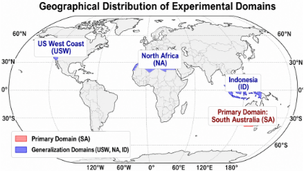
Table 4 empirically checks this residual predictability premise by reporting correlations between residuals and forcing across regions. Table 3 further shows that physical forcing is important: removing ∆Ft turns the method into unguided residual fitting and can degrade performance below the frozen baseline.
5 Experiments
5.1 Study Area
As shown in Figure 3, we evaluate PhyTTA using one primary region and three generalization regions.
Primary Region: South Australia (SA). We choose South Australia as the primary region due to its hydroclimatic variability and sensitivity to large scale modes such as the El Niño-Southern Oscillation (ENSO) and the Indian Ocean Dipole (IOD); we focus on its agricultural zone (bounds in Figure 3).
Generalization Regions. We further evaluate on three regions: (i) US West Coast (USW), a Mediterranean regime where temperature anomalies can intensify drought through elevated evaporative demand [Dai, 2013]; (ii) North Africa (NA), an arid region with strong low frequency regional offsets and limited effective data; and (iii) Indonesia (ID), a tropical monsoon regime dominated by precipitation driven drought dynamics.
5.2 Datasets
We evaluate monthly prediction of the 30-day SPEI series from SPEI-GD [Liu et al., 2024a]. The study period spans 1982/01 to 2018/12. The dataset contains 39 features per time step:
- Target: 30-day SPEI from SPEI-GD [Liu et al., 2024a], sampled monthly.
- Meteorological covariates: 34 variables from the National Centers for Environmental Prediction-National Center for Atmospheric Research (NCEP-NCAR) Reanalysis 1 [Kalnay et al., 1996], including atmospheric dynamics and surface conditions.
| Method | MSE ↓ | Loc. 1 MAE ↓ | R2 ↑ | MSE ↓ | Loc. 2 MAE ↓ | R2 ↑ | MSE ↓ | Loc. 3 MAE ↓ | R2 ↑ |
|---|---|---|---|---|---|---|---|---|---|
| Classical and Recurrent Baselines | |||||||||
| ARIMA | 1.213 | 0.882 | -0.417 | 1.201 | 0.875 | -0.409 | 1.225 | 0.887 | -0.426 |
| ETS | 0.950 | 0.765 | 0.050 | 0.942 | 0.760 | 0.055 | 0.957 | 0.769 | 0.048 |
| LSTM | 0.688 | 0.612 | 0.320 | 0.679 | 0.605 | 0.326 | 0.694 | 0.616 | 0.318 |
| GRU | 0.674 | 0.598 | 0.335 | 0.667 | 0.592 | 0.340 | 0.681 | 0.603 | 0.330 |
| TCN | 0.662 | 0.586 | 0.345 | 0.655 | 0.581 | 0.350 | 0.670 | 0.590 | 0.340 |
| Deep Learning SOTA | |||||||||
| Transformer | 0.537 | 0.554 | 0.451 | 0.510 | 0.581 | 0.522 | 0.745 | 0.655 | 0.365 |
| Autoformer | 0.546 | 0.559 | 0.442 | 0.547 | 0.582 | 0.487 | 0.752 | 0.658 | 0.358 |
| Crossformer | 0.542 | 0.557 | 0.446 | 0.474 | 0.588 | 0.556 | 0.740 | 0.654 | 0.370 |
| DLinear | 0.533 | 0.551 | 0.455 | 0.423 | 0.553 | 0.604 | 0.735 | 0.650 | 0.375 |
| FiLM | 0.558 | 0.569 | 0.430 | 0.529 | 0.597 | 0.505 | 0.760 | 0.662 | 0.350 |
| iTransformer | 0.524 | 0.546 | 0.464 | 0.454 | 0.539 | 0.575 | 0.738 | 0.652 | 0.372 |
| PatchTST | 0.535 | 0.552 | 0.453 | 0.461 | 0.548 | 0.568 | 0.743 | 0.655 | 0.366 |
| TimesNet | 0.550 | 0.562 | 0.438 | 0.489 | 0.572 | 0.542 | 0.754 | 0.659 | 0.356 |
| TSMixer | 0.529 | 0.549 | 0.459 | 0.468 | 0.555 | 0.561 | 0.736 | 0.651 | 0.374 |
| Foundation Models with Test-Time Adaptation | |||||||||
| TimesFM v2.5 (Base) | 0.391 | 0.466 | 0.564 | 0.288 | 0.385 | 0.734 | 0.365 | 0.448 | 0.611 |
| TimesFM v2.5 + RevIN | 0.373 | 0.453 | 0.584 | 0.279 | 0.377 | 0.742 | 0.345 | 0.430 | 0.633 |
| TimesFM v2.5 + TAFAS | 0.350 | 0.434 | 0.610 | 0.265 | 0.367 | 0.756 | 0.325 | 0.414 | 0.654 |
| TimesFM v2.5 + PhyTTA (Ours) | 0.343 | 0.435 | 0.618 | 0.249 | 0.362 | 0.770 | 0.310 | 0.416 | 0.670 |
| Chronos-1 (Base) | 0.398 | 0.456 | 0.558 | 0.304 | 0.379 | 0.718 | 0.442 | 0.466 | 0.532 |
| Chronos-1 + RevIN | 0.415 | 0.459 | 0.540 | 0.296 | 0.374 | 0.726 | 0.433 | 0.458 | 0.540 |
| Chronos-1 + TAFAS | 0.406 | 0.463 | 0.549 | 0.298 | 0.381 | 0.724 | 0.413 | 0.459 | 0.560 |
| Chronos-1 + PhyTTA (Ours) | 0.362 | 0.446 | 0.598 | 0.245 | 0.356 | 0.772 | 0.360 | 0.418 | 0.622 |
| TabPFN-ts v1.0.8 (Base) | 0.472 | 0.503 | 0.532 | 0.444 | 0.490 | 0.550 | 0.411 | 0.471 | 0.573 |
| TabPFN-ts v1.0.8 + RevIN | 0.382 | 0.448 | 0.574 | 0.290 | 0.358 | 0.733 | 0.361 | 0.430 | 0.615 |
| TabPFN-ts v1.0.8 + TAFAS | 0.441 | 0.585 | 0.286 | 0.372 | 0.429 | 0.624 | |||
| TabPFN-ts v1.0.8 + PhyTTA (Ours) | 0.372 0.361 | 0.445 | 0.597 | 0.238 | 0.334 | 0.736 0.781 | 0.353 0.373 | 0.430 | 0.600 |
| Moirai (Base) | 0.402 | 0.469 | 0.552 | 0.309 | 0.386 | 0.712 | 0.462 | 0.476 | 0.508 |
| Moirai + RevIN | 0.522 | 0.568 | 0.418 | 0.672 | 0.549 | 0.382 | 0.494 | 0.559 | 0.474 |
| Moirai + TAFAS | 0.454 | 0.531 | 0.494 | 0.398 | 0.475 | 0.632 | 0.437 | 0.518 | 0.534 |
| Moirai + PhyTTA (Ours) | 0.382 | 0.330 | 0.360 | ||||||
| 0.456 | 0.572 | 0.232 | 0.785 | 0.416 | 0.620 | ||||
- Climate indices: the Southern Oscillation Index (SOI) [Trenberth, 1984], the Indian Ocean Dipole (IOD) [Saji et al., 1999], the Southern Annular Mode (SAM) [Marshall, 2003], and the Niño 3.4 ENSO index [Trenberth, 1997].
We split each series chronologically: the first 70% for training and historical warm up, the next 10% for validation, and the final 20% for testing. The confidence gate τ is selected on the validation split (Sections 3.2 to 3.4) with all remaining scalar settings kept fixed, and reported metrics are computed on the held out test split.
5.3 Baselines and Implementation Sources
To ensure a controlled comparison, we follow the one step rolling protocol of TAFAS [Kim et al., 2025] and compare against classical, neural, foundation model, and test time adaptation baselines. The implementation sources are fixed as follows: ARIMA and ETS use statsmodels [Seabold and Perktold, 2010]; recurrent and neural baselines use PyTorch [Paszke et al., 2019] and the public Time Series Library style implementations [Wu et al., 2023a]; foundation model baselines use the public releases of TimesFM v2.5 [Google Research, 2025], Chronos, Moirai, and TabPFN with the tabpfn time series adapter v1.0.8 [Prior Labs, 2025]. The released repository 1 contains the PhyTTA correction module and the TimesFM runner; auxiliary scripts for the additional foundation backbones, the validation/test split protocol of Section 5.2, and per table reproduction commands are included in the code repo. The following list specifies the baseline families used in Table 1.
- Classical and recurrent models: ARIMA [Box et al., 2015], ETS [Hyndman et al., 2002], LSTM [Hochreiter and Schmidhuber, 1997], GRU [Cho et al., 2014], and TCN [Bai et al., 2018].
- Deep learning SOTA: Transformer [Vaswani et al., 2017],
1 https://github.com/Wentao-Gao/PhyTTA
Autoformer [Wu et al., 2021], Crossformer [Zhang and Yan, 2023], DLinear [Zeng et al., 2023], FiLM [Zhou et al., 2022], iTransformer [Liu et al., 2024b], PatchTST [Nie et al., 2023], TimesNet [Wu et al., 2023b], and TSMixer [Chen et al., 2023].
3. Latest Foundation models: TabPFN [Hollmann et al., 2025] with the tabpfn_time_series adapter (tabpfn-ts v1.0.8) [Prior Labs, 2025], Chronos [Ansari et al., 2024], Moirai [Woo et al., 2024], and TimesFM v2.5 [Das et al., 2024; Google Research, 2025].
4. Test time adaptation: RevIN [Kim et al., 2022] and TAFAS [Kim et al., 2025].
Experimental Protocol. We use rolling one step ahead forecasting (H = 1) with context length L = 288 months and residual buffer N = 100; backbone parameters remain frozen, with hyperparameters as in Eq. (9) and Section 3.2. Within block comparisons compare each frozen base backbone with its PhyTTA corrected version on a shared window; cross block numbers use different windows and are shown for orientation only.
5.4 Performance Evaluation
Main results. Table 1 reports one step ahead (H = 1) SPEI forecasting on three representative SA locations (coordinates in the caption).
PhyTTA achieves 12.3% to 15.1% MSE reductions for TimesFM across the three SA locations with consistent R2 gains, and improves the frozen Chronos, TabPFN, and Moirai backbones at every location. Together with TimesFM, these are 12 backbone location comparisons. RevIN gives modest gains, and TAFAS, which needs inference time gradient updates, edges PhyTTA on MAE at TimesFM Locations 1 and 3 (and beats it on TabPFN Loc. 3). Moirai+RevIN degrades sharply while Moirai+PhyTTA recovers, indicating that physics guided correction is more robust than generic normalization under regional shift.
Cross Regional Generalization. Table 2 shows the evaluation results of TimesFM + PhyTTA on three regions with distinct drought mechanisms. PhyTTA improves MSE in all three, with the largest gains on US West Coast and North Africa and a smaller positive gain on precipitation dominated Indonesia, supporting our hypothesis that correctable residual magnitude depends on regional physical characteristics rather than architecture; relative MSE reduction is the more comparable cross region quantity given different SPEI variance across regions.
| Region | Base (TimesFM) | PhyTTA | Imp. | ||||
|---|---|---|---|---|---|---|---|
| MSE ↓ | MAE ↓ | R2 ↑ | MSE ↓ | MAE ↓ | R2 ↑ | ||
| USWest (USW) | 0.0546 | 0.1770 | 0.9407 | 0.0438 | 0.1565 | 0.9526 | +19.78% |
| North Africa (NA) | 0.0695 | 0.1953 | 0.9291 | 0.0590 | 0.1839 | 0.9398 | +15.11% |
| Indonesia (ID) | 0.2302 | 0.3827 | 0.6207 | 0.2212 | 0.3705 | 0.6354 | +3.91% |
5.5 Analysis
Ablation Study. Table 3 isolates the physics and bias components on SA Location 1. Full PhyTTA performs best;
| Variant | MSE ↓ | Improvement ↑ | Analysis |
|---|---|---|---|
| Base Model w/o Physics w/o Bias Full PhyTTA | 0.3910 0.4080 0.3597 0.3428 | -4.35% +8.01% +12.33% | Baseline Statistical residual fitting only No EMA component Best on this location |
| Region | Corr(rt+1, ∆Pt) | Corr(rt+1, ∆T max t ) | Observed Sensitivity |
|---|---|---|---|
| South Australia | -0.31 | +0.28 | Rainfall sensitive |
| US West Coast | -0.23 | +0.09 | Moderate rainfall sensitivity |
| Indonesia | -0.43 | -0.02 | Precipitation dominated |
| North Africa | -0.41 | +0.31 | Mixed rain and temperature |
removing physical forcing makes the corrected MSE worse than the frozen base, so naive residual fitting can harm a strong frozen model without physics guided inputs. Removing the EMA bias tracker leaves only a partial gain, confirming that the dynamic and static components are complementary.
MechanismVerification. To support Corollary 1's residual predictability premise, we correlate TimesFM residuals with forcing changes (Table 4). Residuals associate meaningfully with ∆Pt or ∆T max t across regions: Indonesia is strongly precipitation driven, North Africa shows a mixed signature on both drivers, and South Australia also shows non trivial correlations on both, consistent with compound drought triggers.
6 Conclusion
We have presented PhyTTA, an inference time residual correction framework for frozen TSFMs on regional drought prediction, combining a dynamic forcing corrector, a static EMA background bias tracker, and a conditional confidence gate. With TimesFM, PhyTTA cuts MSE by 19.78%/15.11% on USW/NA and by 12.3% to 15.1% across three SA locations, and improves the frozen base in all 12 SA backbone location cells (best within block in 11/12). Future work will extend PhyTTA to multi step horizons and uncertainty aware warnings.
7 Social Impact
This work is informed by technical exchange with multidisciplinary teams at CSIRO Environment and CSIRO Technology. PhyTTA targets regional drought early warning settings, where more accurate one step ahead SPEI forecasts can support planning and risk management. Its design uses no backbone parameter updates for low latency deployment and physics guided features for interpretability. The forecasts should not be used as sole decision triggers; deployment requires uncertainty communication, expert review, and decision aligned evaluation.
Acknowledgments
This work was supported by the ARC Discovery Project DP230101122 and the Adelaide University Research Training Program (RTP) Scholarship. We gratefully acknowledge the continued support from the CSIRO Environment and Technology Research Units.
@inproceedings{ijcai2026p795,
  title     = {PhyTTA: Physics-Informed Test-Time Adaptation of Foundation Models for Regional Drought Prediction},
  author    = {Gao, Wentao and Li, Jiuyong and Liu, Lin and Le, Thuc Duy and Liu, Jixue and Chen, Yun and Zhao, Yanchang},
  booktitle = {Proceedings of the Thirty-Fifth International Joint Conference on
               Artificial Intelligence, {IJCAI-26}},
  publisher = {International Joint Conferences on Artificial Intelligence Organization},
  editor    = {Diego Calvanese},
  pages     = {7147--7155},
  year      = {2026},
  month     = {8},
  note      = {AI and Social Good},
  doi       = {10.24963/ijcai.2026/795},
  url       = {https://doi.org/10.24963/ijcai.2026/795},
}
TY - CPAPER TI - PhyTTA: Physics-Informed Test-Time Adaptation of Foundation Models for Regional Drought Prediction AU - Gao, Wentao AU - Li, Jiuyong AU - Liu, Lin AU - Le, Thuc Duy AU - Liu, Jixue AU - Chen, Yun AU - Zhao, Yanchang T2 - Proceedings of the Thirty-Fifth International Joint Conference on Artificial Intelligence, IJCAI-26 PB - International Joint Conferences on Artificial Intelligence Organization PY - 2026 SP - 7147 EP - 7155 DO - 10.24963/ijcai.2026/795 UR - https://doi.org/10.24963/ijcai.2026/795 ER -Copied
Machine-readable versions of this paper, for tools and AI agents:





