
Causal Newton Optimization: Online Calibration with Iterative Local Linear Modeling and Newton Updates
Proceedings of the Thirty-Fifth International Joint Conference on Artificial Intelligence. Main Track. Pages 6380-6388.
https://doi.org/10.24963/ijcai.2026/710
Keywords
- Machine Learning: Optimization
- AI Ethics, Trust, Fairnes: Safety and robustness
- Machine Learning: Online learning
- Uncertainty in AI: Causality, structural causal models and causal inference
Abstract
Optimization in industrial systems often involves calibrating from a semi-optimized state, where global exploration methods like Reinforcement Learning (RL) or Bayesian Optimization (BO) are inefficient or unsafe. We propose Causal Newton Optimization (CNO), an online algorithm that iteratively calibrates inputs under a known causal graph but unknown structural equations. CNO estimates local linear causal effects via additive interventions and employs a log-linear variance regression to robustly guide Newton-based updates. Evaluations on synthetic systems and a chemical plant simulator demonstrate that CNO achieves the best balance between objective improvement and robustness. While traditional PID control suits standard dynamical systems, CNO significantly outperforms RL and BO in complex structural causal models, providing the robust stability vital for safety-critical real-world applications.
- [Aglietti et al., 2020] Virginia Aglietti, Xiaoyu Lu, Andrei Paleyes, and Javier González. Causal Bayesian Optimiza- tion. In International Conference on Artificial Intelligence and Statistics, pages 3155-3164. PMLR, 2020.
- [Åström and Hägglund, 1995] Karl Johan Åström and Tore Hägglund. PID controllers: theory, design, and tuning. The international society of measurement and control, 1995.
- [Astrom and Wittenmark, 1994] Karl Johan Astrom and Bjorn Wittenmark. Adaptive control. Addison-Wesley Longman Publishing Co., Inc., 1994.
- [Bareinboim et al., 2015] Elias Bareinboim, Andrew Forney, and Judea Pearl. Bandits with unobserved confounders: A causal approach. Advances in Neural Information Process- ing Systems, 28, 2015.
- [Camacho et al., 2007] Eduardo F Camacho, Carlos Bor- dons, Eduardo F Camacho, and Carlos Bordons. Con- strained model predictive control. Springer, 2007.
- [Frazier, 2018] Peter I Frazier. A tutorial on Bayesian opti- mization. arXiv preprint arXiv:1807.02811, 2018.
- [Fuller et al., 2021] Sawyer Fuller, Ben Greiner, Jason Moore, Richard Murray, René van Paassen, and Rory Yorke. The Python Control Systems Library (python- control). In 60th IEEE Conference on Decision and Con- trol (CDC), pages 4875-4881. IEEE, 2021.
- [Gultchin et al., 2023] Limor Gultchin, Virginia Aglietti, Alexis Bellot, and Silvia Chiappa. Functional causal Bayesian optimization. In Robin J. Evans and Ilya Sh- pitser, editors, Proceedings of the Thirty-Ninth Conference on Uncertainty in Artificial Intelligence, volume 216 of Proceedings of Machine Learning Research, pages 756- 765. PMLR, 31 Jul-04 Aug 2023.
- [Haarnoja et al., 2018] Tuomas Haarnoja, Aurick Zhou, Pieter Abbeel, and Sergey Levine. Soft actor-critic: Off-policy maximum entropy deep reinforcement learning with a stochastic actor. In International conference on ma- chine learning, pages 1861-1870. PMLR, 2018.
- [Lattimore and Szepesvári, 2020] Tor Lattimore and Csaba Szepesvári. Bandit algorithms. Cambridge University Press, 2020.
- [Lattimore et al., 2016] Finnian Lattimore, Tor Lattimore, and Mark D Reid. Causal bandits: Learning good inter- ventions via causal inference. Advances in neural infor- mation processing systems, 29, 2016.
- [Marlin and Marlin, 1995] Thomas E Marlin and TE Marlin. Process control: designing processes and control systems for dynamic performance, volume 2. McGraw-Hill New York, 1995.
- [Pearl et al., 2016] Judea Pearl, Madelyn Glymour, and Nicholas P Jewell. Causal inference in statistics: A primer. John Wiley & Sons, 2016. [Pearl, 2009] Judea Pearl. Causality. Cambridge University Press, 2009.
- [Sani et al., 2020] Numair Sani, Jaron Lee, and Ilya Shpitser. Identification and estimation of causal effects defined by shift interventions. In Conference on Uncertainty in Arti- ficial Intelligence, pages 949-958. PMLR, 2020.
- [Shimizu et al., 2006] Shohei Shimizu, Patrik O Hoyer, Aapo Hyvärinen, Antti Kerminen, and Michael Jordan. A linear non-Gaussian acyclic model for causal discovery. Journal of Machine Learning Research, 7(10), 2006.
- [Shimizu et al., 2011] Shohei Shimizu, Takanori Inazumi, Yasuhiro Sogawa, Aapo Hyvärinen, Yoshinobu Kawahara, Takashi Washio, Patrik O Hoyer, and Kenneth Bollen. Di- rectLiNGAM: A direct method for learning a linear non- gaussian structural equation model. The Journal of Ma- chine Learning Research, 12:1225-1248, 2011.
- [Sinha and Mishra, 2018] Abhinav Sinha and Rajiv Kumar Mishra. Control of a nonlinear continuous stirred tank reactor via event triggered sliding modes. Chemical En- gineering Science, 187:52-59, 2018.
- [Spirtes and Glymour, 1991] Peter Spirtes and Clark Gly- mour. An algorithm for fast recovery of sparse causal graphs. Social Science Computer Review, 9(1):62-72, 1991.
- James H Stock and Mark W Wat- son. Introduction to econometrics (3rd updated edition). Age (X3), 3(0.22), 2015.
- [Subramanian and Ravindran, 2025] Chandrasekar Subra- manian and Balaraman Ravindran. Causality in bandits: A survey. ACM Computing Surveys, 2025.
- [Süli and Mayers, 2003] Endre Süli and David F Mayers. An introduction to numerical analysis. Cambridge University Press, 2003.
- [Uppal et al., 1974] Ashok Uppal, Willis Harmon Ray, and Aubrey B Poore. On the dynamic behavior of continu- ous stirred tank reactors. Chemical Engineering Science, 29(4):967-985, 1974.
- [Wright et al., 1999] Stephen Wright, Jorge Nocedal, et al. Numerical optimization. Springer Science, 35(67-68):7, 1999.
- [Zeng et al., 2024] Yan Zeng, Ruichu Cai, Fuchun Sun, Libo Huang, and Zhifeng Hao. A survey on causal reinforce- ment learning. IEEE Transactions on Neural Networks and Learning Systems, 2024.
References were extracted automatically from the PDF and may contain errors.
Full text extracted automatically from the PDF; figures, tables and equations may differ. The PDF is the version of record.
1 Introduction
Optimization under Real-World Setting. In many industrial and economic systems, optimization operations are rarely started from scratch. Instead, they typically operate in a semi-optimized state, governed by existing mechanisms such as PID controllers and professional manual control in chemical plants, or established policy guidelines in economics. However, due to complex nonlinear dynamics and unmodeled exogenous disturbances, these systems often suffer from persistent deviations (e.g., steady-state errors or oscillations) from the ideal target [ ˚Astr¨om and H¨agglund, 1995]. Operators attempt to mitigate these errors through manual tuning, typically analyzing operation logs accumulated over a fixed period and adjusting parameters at regular intervals (e.g., monthly maintenance). This scenario, where calibration is performed after collecting a certain amount of data at a fixed frequency, is standard and natural in process industries such as chemical plants. Relying on trial-and-error in this periodic process is labor-intensive and inconsistent.
∗The supplementary appendices and full proofs are available at: https://github.com/nttcom/CNO-Supplementary.
To automate this optimization, methods such as Reinforcement Learning (RL) and Bayesian Optimization (BO) are potential candidates. However, these global optimization approaches generally face the exploration-exploitation tradeoff, requiring extensive exploration to learn the global landscape. In safety-critical systems like chemical plants or healthcare, such exploratory behaviors, especially hard interventions that fix inputs and break existing semi-optimization, are often unacceptable due to safety risks and potential economic losses. Furthermore, real-world systems are often nonstationary; dynamics drift due to equipment aging (e.g., catalyst degradation) or seasonal shifts. Global models (e.g., Gaussian Processes in BO) often struggle to adapt quickly to these shifts and suffer from scalability issues regarding historical data storage.
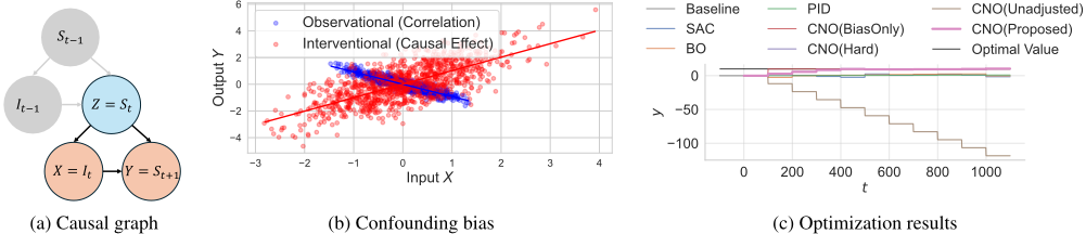
Confounding Bias in Feedback Control. A critical challenge in optimizing such semi-optimized systems is the presence of confounders-variables that influence both the manipulated input and the target output. For instance, in a typical feedback control system, a past system state or an external disturbance affects both the current control input (via existing feedback mechanisms) and the future state of the system (Figure 1a). Ignoring this underlying causal structure leads to biased estimates of the input's true effect on the output (Figure 1b). If an optimizer relies merely on observational correlations rather than causal effects, at worst this confounding bias can flip the apparent direction of the effect, driving a naive optimization algorithm in the completely wrong direction (Figure 1c). We will formally illustrate this phenomenon using a concrete mathematical example in Section 4.
1.1 Proposed Approach
To address these challenges, we propose Causal Newton Optimization (CNO). Unlike global explorers, CNO frames the problem as the online calibration of a continuous input variable to fine-tune an existing system. Our approach rests on three key pillars justified by the calibration setting:
Additive Intervention for Safety. Instead of replacing the existing control logic (hard intervention), we employ additive interventions that superimpose a correction term onto the natural input value. This preserves the system's inherent response mechanisms (e.g., safety feedback loops) and leverages natural fluctuations for estimation, significantly enhancing safety compared to exploration without prior knowledge.
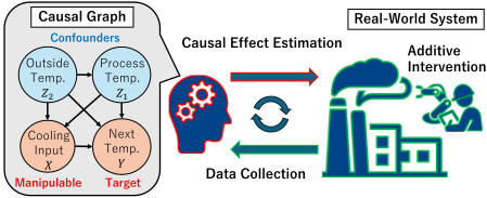
Moreover, CNO's local linear modeling provides high interpretability, allowing operators to understand and trust the optimization process.
Newton's Method for Fast Convergence. We posit that in the neighborhood of a semi-optimal state, system dynamics can be well-approximated by local linear models. By leveraging this inductive bias, CNO estimates local gradients and utilizes Newton's method. This enables CNO to achieve fast convergence based on Newton's method's quadratic characteristics, minimizing the duration of suboptimal operation and adapting rapidly to system drifts without the heavy computational burden of maintaining global models.
Causal Inference for Confounding Adjustment. A critical challenge in this setting is confounding. When using additive interventions, the input remains correlated with upstream variables (confounders). For instance, external temperature might affect both the control input (via existing feedback) and the target outcome. Ignoring this causal structure leads to biased gradient estimates potentially driving the optimization in the wrong direction (as demonstrated in our motivating example). CNO explicitly addresses this by using a known causal graph to perform back-door adjustment, ensuring valid gradient estimation even under confounding.
In this paper, we propose CNO, an algorithm that iteratively estimates local linear causal effects on expectation and variance from online data to update interventions. We introduce a log-linear variance regression to robustly handle heteroscedasticity. Experiments on synthetic nonlinear systems and a continuous stirred-tank reactor (CSTR) simulator demonstrate that CNO achieves faster convergence and higher robustness compared to RL, BO and PID (a standard feedback control method).
2 RelatedWork
2.1 Online Optimization &Control
Reinforcement Learning (RL), such as Soft Actor-Critic (SAC) [Haarnoja et al., 2018], learns optimal policies for dynamical environments through interaction without explicit system models. While flexible as black-box solvers, RL algorithms often suffer from sample inefficiency, requiring sensitive tuning of numerous hyperparameters and manual reward function design. They typically need many trialand-error episodes, often requiring pre-training in simulators to achieve acceptable performance in real-world systems. Bayesian Optimization (BO) [Frazier, 2018] optimizes blackbox objective functions globally by building probabilistic surrogate models, typically Gaussian Processes (GPs). BO focuses on balancing the exploration-exploitation trade-off and can be sample-efficient by explicitly modeling the objective function. However, BO typically scales poorly with highdimensional parameter spaces and increasing historical data, and it requires careful kernel selection for accurate modeling. Bandit algorithms [Lattimore and Szepesv´ari, 2020] also address the exploration-exploitation trade-off but often assume discrete action spaces, making them less effective for continuous parameter tuning. Furthermore, since RL, BO, and Bandits fundamentally require exploratory behavior, safety guarantees are often challenging in real-world applications such as plant engineering. Classical control theories, such as PID control [ ˚Astr¨om and H¨agglund, 1995], typically assume a known dynamical system structure or rely on feedback error correction without learning from online data distributions. Their primary aim is to maintain system stability and track setpoints (exploitation). While Adaptive Control [Astrom and Wittenmark, 1994] can learn data online, and Model Predictive Control (MPC) [Camacho et al., 2007] explicitly can use pre-trained models of dynamics, they generally require accurate system models and may struggle with unmodeled dynamics or complex disturbances.
CNO bridges the gap between these fields and causal inference. Unlike RL, BO, and Bandit, CNO leverages the known causal graph and the inductive bias of local linear approximations around a semi-optimal state, resulting in high sample efficiency without extensive exploration phases. Unlike PID, CNO explicitly handles confounding bias through backdoor adjustment, proactively learning from online data to correct steady-state error that feedback control alone cannot resolve. Moreover, CNO's local linear modeling allows high interpretability and low computational overhead, adapting to trends and distribution shifts.
2.2 Causal Inspired Optimization
Recently, methods integrating causal inference with online optimizations are emerging. Surveys are available in [Zeng Initial Value Optimal Value Errors Data Collecting Third ···
First Second
intervention
- (a) Repeating interventions
(b) Problem setting overview
𝑐!
Causal Effect
𝜇′(𝑐!)
Expectation
𝜇(𝑐!)
𝑐!"#
Optimal
Intervention
𝑐∗
𝑐!"%
- (c) Local estimation and Newton's method
Figure 2: Overview of the proposed method. (a) Optimization reducing errors by repeated interventions. (b) Problem settings of optimization. Collected data by intervention is available online. (c) Combination with local linear estimation of causal effects and Newton's method.
et al., 2024; Subramanian and Ravindran, 2025].
Causal Optimization for Efficient Intervention Exploration. Lattimore et al. [2016] extended the multi-armed bandit problem by considering causal relationships between arms to identify optimal interventions. Similarly, Causal Bayesian Optimization (CBO) [Aglietti et al., 2020; Gultchin et al., 2023] propose causal-aware Gaussian Processes model to simultaneously identify the optimal intervention set and values. These methods primarily focus on the explorationexploitation trade-off and address the combinatorial explosion of intervention variables utilizing known causal relationships. In contrast, CNO targets the calibration of a specific continuous variable in a semi-optimized system, focusing on fast convergence rather than global exploration.
Causal Optimization for Adjustment of Confounding. Bareinboim et al. [2015] focused on adjusting confounding bias in multi-armed bandit problems. They demonstrated that conventional bandit algorithms perform sub-optimally when unobserved confounders influence both the intervention (arm selection) and the outcome. Crucially, they utilized not only interventional data but also natural observational data to extract information about unobserved confounders, improving algorithm efficiency. CNO shares the aim of adjusting confounding bias and utilizing natural observational data (via additive interventions). However, while Bareinboim et al. address the discrete arm selection problem with explorationexploitation, CNO focuses on continuous variables tuning with fast convergence, and uses inductive bias from local linear approximations around a semi-optimal state.
3 ProposedMethod
3.1 Problem Setting
We assume that the data consist of continuous variables and follow a structural causal model (SCM). In an SCM, the causal generative process of the data is described by structural equations, and the causal relationships are represented by a directed graph [Pearl, 2009; Pearl et al., 2016]. We assume a known, acyclic causal graph G with unknown functional forms of the structural equations. For P ∈ N variables, the structural equations are:
where pai is the set of direct causes (i.e. parents) of Vi given from the causal graph G, and fi is an unknown deterministic function. The exogenous variable Ui is a random variable determined independently of the structural equations and representing unobserved disturbances. The endogenous variable Vi is a random variable generated from structural equations. Let V = {Vi | i = 1, 2, . . . , P}. We define Y (∈ V ) as a target variable for optimization and X (∈ V ) as a variable manipulable through interventions. We evaluate Y against a constant reference value (setpoint) Y ∗ ∈ R using the standard squared error, L(Y ) = (Y - Y ∗ )2 .
Calibration Setting via Additive Intervention. We assume the system is currently operating in a semi-optimized state governed by existing mechanisms (e.g., manual control or feedback loops)[ ˚Astr¨om and H¨agglund, 1995; Marlin and Marlin, 1995; Sinha and Mishra, 2018].
Assumption 1 (Calibration Setting for Semi-Optimized). Let Xnat be the natural value of X determined by the structural equation Xnat = fX(paX ,UX). We assume Xnat is semioptimized for L(Y ), e.g. minimization of its expectation, minfX (E[L(Y )| do(X = Xnat)]). Then the outcome under the natural state, Y |do(X = Xnat), lies within a neighborhood of Y ∗ where G(c) is locally convex and the GaussNewton approximation holds.
Rather than the standard hard interventions, we calibrate the existing Xnat using an additive intervention [Pearl et al., 2016; Sani et al., 2020] with a correction term c ∈ R:
This intervention in (2) shifts the mean by c, preserving the dependence of X on exogenous noises UX and parents paX , while standard hard interventions fix X to a constant a and remove the causal links from parents to X. This setting ensures safety by maintaining the system's reaction to disturbances and allows us to leverage the preserved natural variance of Xnat for estimating local causal effects. Furthermore, since the system is in a neighborhood of an optimal state, the nonlinearity of the system is often relatively relieved. This property justifies the use of local linear approximations for online estimation. The optimization of the correction term c is formulated as:
𝑋 = 𝑐
𝒕
𝑌|add(𝑋, 𝑐)
Optimal
Value
𝑌∗
Bias
𝐺#(𝑐!)
Variance
𝐺%(𝑐!)
:Observed Data Since fi and Ui are unknown, the expectation in (3) cannot be computed analytically. We consider an online setting where system observations are obtained at time steps t ∈ N:
However, the correction term c is not updated at every step; instead, c is held constant over a fixed interval T ∈ N, to collect multiple data points for estimation. We assume that the data points v(t) are i.i.d. samples generated from a timeinvariant SCM under the additive intervention. Thus, the distributions of variables depend on time t only through the updated correction term c. Let m = 0, 1, . . . be the iteration index. The data batch Dm collected under the m-th correction term cm is defined as:
After obtaining Dm, we estimate local statistics to calculate the next correction term cm+1. cm+1 will be applied to the system to collect the subsequent batch Dm+1.
3.2 Derivation of Optimization Algorithm
Newton's method. We employ a Newton-based algorithm to solve the optimization problem in (3). Defining the derivative of the objective function as g(c) := G′ (c), Newton's method seeks the root g(c) = 0 via the following update rule:
A Newton-based approach provides clear interpretability of the algorithm's behavior, theoretical basis of fast convergence (approximately quadratic). Moreover it aligns with the linear causal modeling ((9), etc.). See Supplementary Material Appendix A, and [S¨uli and Mayers, 2003] for detailed assumptions and the statement.
Local Convexity. Although global convexity of G(c) is needed in Newton's method optimization, it is not guaranteed for general nonlinear functions. However, our problem setting calibration of an existing optimization (Assumption 1) justifies the assumption of local convexity.
Lemma 1 (Local Convexity under Calibration Setting). Under the assumption of semi-optimized setting (Assumption 1), the initial correction term c0 = 0 is within a sufficiently small neighborhood of strict local optimum of c∗ . In this region, the objective function G(c) is assumed to be convex and twice differentiable. Under this assumption, the standard convergence properties of Newton's method apply (see Supplementary Material Appendix B for details).
Decomposition of Objective Function. The expectation in (3) can be transformed by an approach analogous to the standard bias-variance decomposition:
where µ(c) = E [Y | add (X, c)]. Note that if all structural equations fi are linear, the variance G2(c) remains constant regardless of c, while general nonlinear structural equations lead to G2(c) varying with c.
Since the distribution p(Y | add(X, c)) is unknown, we cannot analytically compute G(c) or its derivatives. In our proposed method, we approximate and estimate the terms g(cm) = g1(cm) + g2(cm) and g′ (cm) = g′1 (cm) + g′2 (cm) to compute the update in (4).
Derivatives of Squared Bias. We first consider the squared bias termG1(c) and its derivatives.
Lemma 2 (Approximation of the Derivative g′1 (c)). Under the calibration setting (Assumption 1), µ(c) is expected to be sufficiently close to Y ∗ (i.e., the bias is small) such that (µ(c) - Y ∗ )µ′′ (c) is negligible compared to µ′ (c)2 . Therefore, the following equation and approximation hold:
The approximation (7) ignores second-order derivative, so aligns with the linear causal modeling ((9), etc.).
Remark. The approximation in (7) is equivalent to the strategy employed in the Gauss-Newton method (see [Wright et al., 1999] for details), which is widely established for solving nonlinear least squares problems. While the standard GaussNewton method is typically designed for static optimization with known parametric functions, our approach extends this framework to an online stochastic optimization setting where functions are unknown and must be estimated via causal inference.
Local Causal Effect Estimation. To calculate (6) and (7), we need to estimate the derivative µ′ (c) = ∂ ∂c E[Y | add(X, c)], which represents the local causal effect of X on Y under the additive intervention. Standard causal inference typically assumes hard interventions do(X = a), which fix X to a specific value. While each derivative estimated under additive and hard interventions differs in general nonlinear cases, it becomes equivalent in linear models.
Lemma 3 (Equivalence of Linear Hard and Additive Causal Effects ). Under the setting of a constant linear causal effect wYX = ∂ ∂a E[Y | do(X = a)], the local causal effect of X on Y under hard interventions is equal to that under additive interventions:
Thus, under the assumption of local linearity (discussed in Lemma 4), we can approximate the causal effect under additive interventions using the standard back-door adjustment (discussed in Proposition 1) under hard interventions.
In linear SCMs, the causal effect wYX is constant and can be estimated via the back-door adjustment [Pearl, 2009; Pearl et al., 2016]. In the back-door adjustment, using a set of covariates Z that satisfies the back-door criterion as explanatory variables in addition to X, the Ordinary Least Squares (OLS) can consistently estimate the causal effect. Specifying the back-door criterion needs the known causal graph G. Refer to the detailed definition in Supplementary Material Appendix C.
Proposition 1 (Back-door Adjustment in Linear Case). Assume a linear SCM with known causal graph where variables Z ⊂ V \ {X, Y } satisfy the back-door criterion relative to (X, Y ). Consider the linear regression of Y on X and Z:
where we assume E[ϵ] = 0 (absorbed into w0). Then, the regression coefficient wYX identifies the constant causal derivative wYX = ∂ ∂a E [Y | do (X = a)]. The OLS estimator ˆwYX is consistent for wYX as the sample size increases [Stock and Watson, 2015].
Local Linearity of Structural Equations. Since the structural equations fi in (1) are generally nonlinear, we employ a local linear approximation around the current intervention value cm.
Lemma 4 (Linearization over Structural Equations). Assuming fi are twice differentiable, the deviation of ξ = (pai, Ui)T and Hessian ∇2 fi is sufficiently small, the entire SCM can be approximated by a linear model locally. (see Supplementary Material Appendix D for formal conditions and proofs)
Considering all the above discussion, the approximated estimators for µ′ (c) are given as ˆµ′m := ˆµ′ (cm) = ˆwYX. The expectation µ(cm) is estimated by the sample mean of observed Y values under additive interventions add(X, cm), ˆµm := 1 T ∑(m+1)T t=mT+1 y(t) . Considering (6) and (7), we get following estimators:
Approximated Derivatives of Variance
Estimating the derivatives of the variance term, g2(c) and g′2 (c), is challenging. The naive finite differences often leads to numerical instability, particularly when the intervention step size |cm-cm-1| is small in the convergence stages of the algorithm. To overcome this, we propose a robust estimation method based on a local log-linear approximation.
Instead of estimating variance and derivatives directly, we assume the conditional variance locally follows a log-linear relationship with the intervention c, i.e., lnG2(c) ≈ ω0 + ωc. Under this assumption, the derivatives satisfy g2(c) = ωG2(c) and g′2 (c) = ω2G2(c) (see Supplementary Material Appendix E for derivation). This formulation ensures consistency with the positivity of variance. To estimate the coefficient ω, we employ heteroscedastic regression using the residuals r(t) = y(t) - ˆw0 - ˆwYXx(t) - ˆw⊤ YZ z(t) . Note that, although the sample mean ˆµm is sufficient for an unbiased estimation of g1(c) and biased but stable estimation of g′1 (c), using it for residual estimation introduces crucial bias due to the local mean shift. Therefore, we use regressionbased residuals (see Supplementary Material Appendix F for details). Thus, we solve the following regression problem:
Using the same adjustment set Z as in the regression, confounding biases are theoretically adjusted for the variance as well [Pearl, 2009; Pearl et al., 2016] (see Supplementary Material Appendix G). Moreover, the OLS (11) provides a consistent and unbiased estimator of the local variance coefficient ωYX, although biased estimator for the intercept ω0 and the variance G2(c) (see Supplementary Material Appendix H). Finally, combining ˆωYX with the current variance estimate ˆG2(cm) := 1 T ∑(m+1)T t=mT+1 (r(t) )2 , we compute the derivatives for the Newton update as:
We provide a detailed discussion about other variance estimators in Supplementary Material Appendix J.
Resulting Update Equation
Considering (4) ∼ (12), the algorithm we developed for the proposed method is given as the following update equation:
Note that initial correction term is set as c0 = 0. If the structural equations are completely linear or ignoring G2(c), where ˆ g2,m = ˆ g′2,m = 0, we can obtain the following more interpretable form: cm+1 - cm = Y ∗-ˆµm ˆµ′m . This form indicates the division of the offset Y ∗ - ˆµm by the local causal effect ˆµ′m, which is illustrated in the first concept of Figure 2c. The pseudo-code of the entire algorithm is summarized in Supplementary Material Appendix I.
4 Numerical Experiments
To evaluate the effectiveness of our proposed method, Causal Newton Optimization (CNO), we conducted a series of experiments across three distinct environments with varying complexities. We compare CNO against representative algorithms from system control and online optimization. In every experiment, we set the time interval for each intervention as T = 100.
Linear SCM: Confounding Bias in Feedback Control. To formally illustrate the confounding bias discussed in Section 1, we evaluate a simple linear SCM representing the feedback control system depicted in Figure 1a. Consider a state variable to be controlled S(t) . In a typical semi-optimal steady-state, S(t) fluctuates around a constant ˜ r (= a reference value r + steady-state error). The system dynamics, including the feedback control input I (t) , can be modelled as:
where Kp = 0.5, α = 1.0, β = 1.0, σUZ = 1.0, σUX = 0.1, and σUY = 0.1, r = Y ∗ = 10.0. For simplicity, variables are assumed centered. We aim to optimize the output Y = S(t+1) by manipulating the input X = I (t) , adjusting for Z = S(t) .

While the true interventional coefficient fromX → Y is α, the unadjusted estimation yields the observational coefficient:
This approximation holds when σUZ ≫ σUX . Crucially, when β/Kp > α, which holds for the adopted parameters, this apparent coefficient becomes negative (ˆα < 0), mathematically demonstrating the confounding bias (Figure 1b). The total number of interventions is M = 10.
Complex Synthetic Environment. We randomly generated 100 different SCMs with P = 10 variables and random Directed Acyclic Graphs (DAG), where each edge is created with a probability of p = 0.3 after arranging a random causal order to prevent cycles. If there is no back-door set under a generated graph, the graph is rejected and resampled. The functional forms in the structural equations consisted of linear combinations of parental variables and their polynomials, scaled to be order 1, as follows:
where aik and bij are constant values sampled from the distribution: Uniform([-1,-0.5] ∪ [0.5, 1]), and K = 3 as the range of Y is [-∞,∞](∋ Y ∗ ). σi is randomly sampled from Uniform([0.1, 0.3]) so that 3σi ≤ 1, guaranteeing P(|Ui| ≤ 1) > 0.997. The total number of interventions is set as M = 100, the optimal value is set as Y ∗ = 0 for scalefree evaluation. Note that in this environment, Xnat is not in a semi-optimized state under a existing mechanism, but randomly sampled. This setup tests the algorithms' robustness to varying and complex nonlinear relationships and violations of Assumption 1.
CSTR Simulator. To assess practical applicability in realworld scenarios, we used a Continuous Stirred-Tank Reactor (CSTR) simulator, a well-known benchmark in process control and machine learning tasks with strong nonlinear dynamics [Uppal et al., 1974; Marlin and Marlin, 1995; Sinha and Mishra, 2018]. The implementation used python control library [Fuller et al., 2021]. In this environment, the goal is to regulate the reactor temperature by manipulating the cooling jacket temperature. We set the situation that PID control is already applied but the accuracy is not sufficient. PID control is a method typically suitable for linear systems, not for nonlinear systems such as CSTR, thus this setting is reasonable. Algorithms can start from steady-state by using a stabilization period without interventions. Note that this setting is consistent with the assumption of semioptimized state (Assumption 1). See Supplementary Material Appendix N for details. The total number of interventions is set as M = 100, the optimal value is set as Y ∗ = 328.0[K] under physical limitations.
Compared Methods. Some representative methods from classical system control and modern online optimization were selected to compare with our proposed method, CNO. Compared methods are applied to under the same conditions as CNO, such as the same T, M, and additive intervention settings. (Outer Loop) PID Controller: As a representative of classical system control, we implemented a velocity-form PID controller. PID control gain parameter was well handtuned. Further details are provided in Appendix M. Note that in CSTR Simulator, another PID control with different parameters and a different intervention interval is already applied to the plant. Soft Actor-Critic (SAC): As a state-ofthe-art model-free reinforcement learning method, we used SAC. The specific architecture and reward function design are described in Appendix L. Bayesian Optimization (BO): We also implemented a BO method using Gaussian Process (GP) regression as a surrogate model and Lower Confidence Bound (LCB) as an acquisition function. Note that SAC and BO have sensitive intervention range parameters. We use ±5σ (σ is standard deviation) of initial state Xnat as the intervention range. Proposed Methods (CNO Variants): To analyze the contribution of each component of our proposed method, we evaluate several CNO variants with different variance estimators and intervention types (hard or additive). Note that, hard interventions require excitation noise to identify the causal effect, while additive does not. And there are variants that do not perform back-door adjustment (Unadjusted) and that only adjust squared bias G1(c) (BiasOnly).
Evaluation Metrics. We assess the performance of all algorithms using the following metrics. Objective Function, Squared Bias, Variance: We evaluate the time-averaged values of the objective function G(c), which is equivalent to the Mean Squared Error (MSE) from Y ∗ over the experiment's duration, and the squared bias G1(c) and variance G2(c). Ratio of Objective Functions: The ratio of each objective function G(c), G1(c), G2(c) before and after applying the algorithm (after/before). Thus a value less than 1 indicates improvement. Improved Sample Proportion: The proportion of experimental trials in which the ratio of G(c) is less than 1, excluding any trials that exhibited divergence. Steady-State (SS) Metrics: The Objective Functions, Ratios, Improved Sample Proportion in the stable state after the transient response has settled. These are computed by taking the last 10% of overall time length (M × T) from the time series of the target variable Y .
| Complex Env. | CSTR Env. | ||||||
|---|---|---|---|---|---|---|---|
| Obj. Ratio (SS) ↓ | Bias2 Ratio (SS) ↓ | Var. Ratio (SS) ↓ | Imp. ↑ | Imp. (SS) ↑ | Obj. Ratio (SS) ↓ | Imp. (SS) ↑ | |
| SAC | 1.02 ± 0.137 | 1.09 ± 0.762 | 1.01 ± 0.0625 | 45/100 | 53/100 | 0.682 ± 0.464 | 88/100 |
| BO | 1.01 ± 0.0783 | 1.01 ± 0.167 | 1.00 ± 0.0631 | 51/100 | 47/100 | 1.26 ± 1.44 | 69/100 |
| PID | 0.998 ± 0.0728 | 1.01 ± 0.221 | 1.00 ± 0.0619 | 49/100 | 52/100 | 0.427 ± 0.0453∗ | 100/100 |
| CNO (BiasOnly) | > 1020 | > 1020 | > 1020 | 61/99 | 72/99 | 0.443 ± 0.0546 | 100/100 |
| CNO (Hard) | 0.943 ± 0.26 | 0.925 ± 0.524 | 1.00 ± 0.0696 | 60/100 | 66/100 | 141 ± 72.8 | 0/100 |
| CNO (Unadjusted) | 837 ± 8320 | 57.9 ± 570 | 1240 ± 12300 | 76/100 | 77/100 | 28.7 ± 48.6 | 72/100 |
| CNO (Proposed) | 0.762 ± 0.225∗ | 0.516 ± 0.4 | 1.06 ± 0.347 | 85/100 | 84/100 | 0.433 ± 0.0459∗∗ | 100/100 |
Results. Linear SCM: As shown in Figure 1c, only our CNO considering confounding successfully calibrated the target variable Y . CNO(Unadjusted) drove the optimization in the wrong direction due to the confounding effect. Complex Synthetic Environment: As Table 1 shows, CNO is superior to other methods in terms of the Improvement Ratio of Objective Function and Squared Bias, as well as the Improved Sample Proportion, while maintaining comparable variance. Figure 3a shows a representative trial where only CNO successfully optimizes the target variable while other methods struggle in complex SCMs. CSTR Simulator: Looking at the results in Figures 3b and 3c and Table 1, our CNO demonstrates superior performance to SAC and BO, and performs as well as PID in steady state and Improved Sample Proportion.
Overall, CNO achieves the best balance between objective improvement and robustness. While the CSTR environment favors PID control, CNO excels in complex environments following general SCMs, demonstrating the robust stability vital for safety-critical real-world applications.
5 Discussion and Limitations
Local Optimization. Since CNO employs a Newton-style update, it is inherently a local optimizer designed for the calibration of semi-optimized systems (Assumption 1), rather than global exploration. Consequently, convergence to local optima or transient overshoot may occur if the system is initialized far from the optimal basin of attraction.
Dependence on Known Causal Structure. Accurate gradient estimation relies on the correctness of the causal graph G for confounding adjustment. While CNO is robust to parametric uncertainty, structural misspecification (e.g., unmeasured confounders) can bias estimates. Addressing unknown structures via causal discovery [Spirtes and Glymour, 1991; Shimizu et al., 2006; Shimizu et al., 2011] remains a future challenge. Furthermore, the assumption that all system variables are observed (causal sufficiency) is implicitly adopted, which is a very strong condition. Therefore, robustness against other factors such as unobserved confounders must also be verified.
Univariate Limitation. The current formulation focuses on a single manipulatable variable. Extending CNO to multivariate interventions requires estimating the full Hessian matrix (including off-diagonal interaction terms), which significantly increases sample complexity and computational cost (corresponding to the quasi-Newton methods).
Approximation and Dynamics. The Gauss-Newton approximation omits the second-order term (µ(c) - Y ∗ )µ′′ (c), which is theoretically valid only when residuals are small. Furthermore, accurate causal effect estimation assumes the system reaches a quasi-steady state within the intervention interval T; rapid non-stationary drifts or insufficient settling times may violate this assumption.
6 Conclusion
In this paper, we proposed Causal Newton Optimization (CNO), an online algorithm designed for the calibration of semi-optimized systems. Unlike global exploration methods, CNO leverages prior knowledge of existing semioptimization and iterative local linear causal modeling and Newton-based updates to achieve fast convergence while maintaining safety through additive interventions. Crucially, CNO explicitly handles confounding bias and incorporates a log-linear variance regression to minimize target variance. These result in robust performance. Our evaluation demonstrates that CNO achieves the best balance between objective improvement and robustness. While standard dynamical systems favor traditional PID control, CNO significantly outperforms RL and BO methods, and excels in complex environments governed by general SCMs. This highlights CNO's robust stability for unknown systems, which is vital for safetycritical, real-world applications.
Ethical Statement
The proposed Causal Newton Optimization (CNO) aims to enhance the efficiency and safety of industrial and economic systems by providing a robust online calibration framework. By employing additive interventions, CNO explicitly preserves existing safety mechanisms and feedback loops, significantly reducing the risks associated with raw exploration in safety-critical environments such as chemical plants. Furthermore, the use of local linear causal modeling enhances the interpretability of the optimization process, allowing human operators to monitor and verify algorithmic updates effectively. While the automated nature of CNO could potentially lead to over-reliance on the system, we emphasize that it is designed to complement existing professional control and should be integrated with appropriate monitoring safeguards to mitigate risks from extreme non-stationary drifts.
Acknowledgements
This work was supported by JST CREST Grant Number JPMJCR22D2 and NTT DOCOMO BUSINESS Inc. The authors would like to thank our colleagues at NTT DOCOMO BUSINESS for their insightful discussions and continuous support throughout this project. The authors are also grateful to Shiga University for providing the academic environment and resources that facilitated this research.
@inproceedings{ijcai2026p710,
  title     = {Causal Newton Optimization: Online Calibration with Iterative Local Linear Modeling and Newton Updates},
  author    = {Fujiwara, Daigo and Izumitani, Tomonori and Shimizu, Shohei},
  booktitle = {Proceedings of the Thirty-Fifth International Joint Conference on
               Artificial Intelligence, {IJCAI-26}},
  publisher = {International Joint Conferences on Artificial Intelligence Organization},
  editor    = {Diego Calvanese},
  pages     = {6380--6388},
  year      = {2026},
  month     = {8},
  note      = {Main Track},
  doi       = {10.24963/ijcai.2026/710},
  url       = {https://doi.org/10.24963/ijcai.2026/710},
}
TY - CPAPER TI - Causal Newton Optimization: Online Calibration with Iterative Local Linear Modeling and Newton Updates AU - Fujiwara, Daigo AU - Izumitani, Tomonori AU - Shimizu, Shohei T2 - Proceedings of the Thirty-Fifth International Joint Conference on Artificial Intelligence, IJCAI-26 PB - International Joint Conferences on Artificial Intelligence Organization PY - 2026 SP - 6380 EP - 6388 DO - 10.24963/ijcai.2026/710 UR - https://doi.org/10.24963/ijcai.2026/710 ER -Copied
Machine-readable versions of this paper, for tools and AI agents:





