Finding Simple Shortest-Paths via Centroids

1 Introduction

A well-studied problem in Artificial Intelligence consists of finding the shortest path in a weighted digraph G between two vertices s and t, given either implicitly or explicitly, e. g. [Dijkstra, 1959; Hart et al., 1968]. As observed by [Eppstein, 2016], many real-world problems are only approximately modeled by these techniques, and the variant which consists of computing an arbitrary number, k, of shortest paths seems to have wider applicability-see [Shibuya and Imai, 1997; Arita, 2000; Xu et al., 2012]. In one variant, paths are allowed to be non-simple [Eppstein, 1998], while in the variant under consideration in this paper, all paths are required to be simple. The latter was originally studied by Hoffman and Pavley [1959], and the first attempt to solve it effectively was done by Clarke et. al. [1963]. However, the first algorithm whose computational upper bound increases only linearly with the value of k was authored by Yen [1971], later improved through the use of specific data structures, yielding a worst-case time complexity of O(kn(m+n log n)) [Lawler, 1972]. This algorithm performs an arbitrary number of Dibeen made to obtain better results. For example, Hershberger et. al. [2007] propose using a replacement path algorithm to linearly improve practical performance, while Feng [2014] tries to avoid some Dijkstra calls by means of node classification. However, it is the consideration of sidetrack edges [Eppstein, 1998] which has proven to provide the best improvements in practice resulting in the algorithm SB [Kurz and Mutzel, 2016]. This algorithm was later improved by Al Zoobi et. al. [2020] who proposed a modification that speeds it up by a factor of 1.5×/2×, resulting in the algorithm SB*.

Remarkably, all these algorithms still conduct an arbitrary number of Dijkstra searches to solve the problem, and are observed to be quite memory-demanding. Also, to the best of the authors' knowledge, all of these algorithms have only been tested over graphs given explicitly, and none of them have been coupled with heuristics, limiting their applicability to harder problem instances. In this paper, we suggest the use of centroids, instead of sidetrack edges, to efficiently solve the k simple shortest-paths problem. Our contribution, sBELA∗ , conducts just a single search over graphs given either implicitly or explicitly, and can be coupled with heuristics with no additional modification. It achieves a dramatic reduction in runtime compared to SB*, while also requiring significantly less memory.

This paper is arranged as follows: the next section introduces some relevant definitions; Section 3 introduces some background, providing a high-level description of BELA∗ , the current state-of-the-art for the computation of non-simple shortest paths. The next two sections discuss ways to adapt it to the simple path variant. A simplistic (yet often used) approach is presented first, and then a smarter approach, which is the core of our contribution, sBELA∗ . The paper ends with a discussion of several experiments and conclusions.

2 Definitions

Given a directed graph G(V,E) characterized by its set of vertices V and set of edges E = {eu,v = u → v : u, v ∈ V }, let s and t denote the start and goal vertices respectively, between which an arbitrary number k of simple distinct shortest-paths must be found. A path π is defined as a concatenation of vertices π⟨n0, n1, n2, . . . , nℓ⟩ such that eni-1,ni ∈ E, 0 < i ≤ ℓ. If s = n0 and t = nℓ then π is a solution path, or an s-t path. π is said to be simple if and only if it is loopless, i.e., it contains no repeated vertices, and it is said to be non-simple otherwise. The edges are weighted with non-negative integers, where ω(ni-1, ni) denotes the cost of traversing the edge eni-1,ni . Thus, the cost of a path π is defined according to the additive model as

context or it is irrelevant, the same cost can also be denoted as g(ni) if and only if the path starts at the start vertex, s and ends at vertex ni. Analogously, gb(ni) denotes the cost of a

and only if nℓ = t. As it will be promptly shown, there might be many different paths with different costs between ni and t and thus, gb(· ) is defined as a set of distinct costs. Following the previous definitions, g∗ (ni), and g∗ b (ni) denote the cost of an optimal path from the start vertex, s to ni, and from ni to t, respectively. A path π is said to be optimal if and only if C(π) ≤ C(π′ ) for every solution path π′ , and is termed as suboptimal otherwise. The set of all solution paths (either optimal or suboptimal) in G is denoted as Gπ, and the set of all paths which are suboptimal is denoted as G′π , G′π ⊂ Gπ.

Definition 1. Given s, t ∈ V , a top-k set of shortest simple s-t paths is a set Π of pairwise distinct (i. e., paths that differ in at least one vertex) simple s-t paths such that |Π| = k, and C(π) ≤ C(π′ ) for every s-t path π ∈ Π and s-t path π′ /∈ Π.

Heuristic functions are denoted as h(· ). They provide an estimate of the unique cost of an optimal path to the goal. A heuristic function is said to be admissible if and only if h(n) ≤ g∗ b (n) for every node n. Note that this definition refers to nodes instead of vertices, which are defined in turn, as the representation of a unique path from s to its corresponding vertex, such that the same vertex can be represented with multiple nodes in a search algorithm. A heuristic function is said to be consistent if and only if h(n) - h(n′ ) ≤ ω(n, n′ ), for every node n, where n′ is any descendant of it.

A central concept in many k shortest-path algorithms (such as Eppstein's Algorithm [Eppstein, 1998], K∗ [Aljazzar and Leue, 2011], SB [Kurz and Mutzel, 2016] or SB* [Kurz and Mutzel, 2016]) is that of sidetrack edges:

Definition 2. Let T denote a shortest path tree with s as its source, e.g., the shortest path tree developed by either Dijkstra or A∗ . Every edge in G\T is called a sidetrack edge; otherwise, it is called a tree edge.

In particular, any edge incident on an already expanded vertex, i. e., a duplicate, is always a sidetrack edge. There are two types of sidetrack edges of interest. Given a sidetrack edge eu,v, either g∗ (v) = g∗ (u) + ω(u, v), or g∗ (v) < g∗ (u) + ω(u, v), since v was expanded before. In the first case, the edge eu,v provides an alternative optimal path to get to v; whereas in the second case it represents a suboptimal path. Note that if g∗ (v) = g∗ (u)+ω(u, v) then whether eu,v is a sidetrack edge or a tree edge solely depends on which is discovered first, which in turn depends on the tie-breaking policy. Instead, if g∗ (v) < g∗ (u) + ω(u, v), then eu,v is always a sidetrack edge, since it would have been discarded by Dijkstra's or A* for being a duplicate with a higher cost.

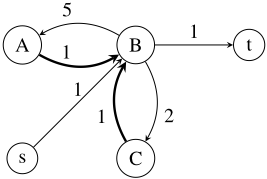
Example 1. Figure 1 shows a graph with two sidetrack edges, namely eA,B and eC,B, all the others being tree edges, e.g., eA,B is a sidetrack edge because g∗ (B) = 1 < g∗ (A) + ω(A, B) = 6 + 1 = 7. ✷

Clearly, the existence of at least one sidetrack edge is both a necessary and sufficient condition for the existence of alternative paths, and many algorithms have used this notion in one form or another. Its importance for our algorithm stems from the fact that it can be used to divide suboptimal paths in a specific manner. In short, the necessary and sufficient condition for a suboptimal path to exist, is that it must contain at least one sidetrack edge of the form g∗ (v) < g∗ (u) + ω(u, v). Hence, any suboptimal solution path π⟨s = n0, n1, n2, . . . , nℓ = t⟩ can be decomposed into a prefix and a suffix, via a sidetrack edge eni-1,ni ∈ π of this type, for any i with 0 < i ≤ ℓ as follows: Let ni be the first node in π which verifies g∗ (ni) < g∗ (ni-1) + ω(ni-1, ni), then:

• ϕ⟨s = n0, n1, . . . , ni-1⟩ is the prefix, possibly empty.
• σ⟨ni, ni+1, . . . , nℓ = t⟩ is the suffix, possibly empty.
• The edge eni-1,ni ∈ π is a sidetrack edge.

Example 2. The suboptimal (non-simple) path ⟨s, B, A, B, t⟩ in Figure 1 is split via the sidetrack edge eA,B into the prefix ⟨s, B, A⟩ and the suffix ⟨B, t⟩. ✷

In contrast to other algorithms which only use the notion of the sidetrack edge, Linares L´opez and Herman [2024] advocate the adoption of a related notion expounded therein for computing k non-simple shortest paths more efficiently:

Definition 3. A centroid z is defined as a tuple (eu,v,Cz), where eu,v ∈ E is a sidetrack edge and Cz is its overall cost.

Centroids induce a partition over the set of all suboptimal paths G′π , i.e., every suboptimal solution path π′ ∈ G′π belongs to one and only one equivalence class defined by a centroid z. As a consequence, the computation of all suboptimal solution paths in Π is equivalent to the computation of ⋃ z∈Z �z�

where Z is the set of all centroids with cost less than or equal to the cost of the k-th solution path, and �z� is the set of all paths corresponding to centroid z. It is highlighted, however,

Algorithm 1: Pseudocode of BELA∗ /sBELA∗

Require: A graph G = (V, E) and two designated vertices s, t Ensure: Solution set Π with k shortest paths 1: CLOSED←∅, Z ←∅ 2: OPEN← {s} with g(s) = 0 3: while OPEN̸= ∅ do 4: n← POP(OPEN) 5: while ∃z ∈ Z such that Cz ≤ f(n) do 6: z ← POP(Z) 7: Π ← Π ∪ GETPATHS(z) 8: if |Π| ≥ k then 9: return Π 10: if n = t then 11: Insert ⟨ept,t, g(n)⟩ into Z 12: continue 13: if n ∈ CLOSED then 14: Insert epn,n into CLOSED (where epn is the parent of n) 15: for every gb-value in n do 16: Insert ⟨epn,n, g∗ (pn) + ω(pn, n) + gb⟩ into Z 17: continue 18: Insert n into CLOSED 19: for each ci ∈ CHILDREN(n) do 20: g(ci) ← g(n) + ω(n, ci) 21: Insert ci into OPEN 22: while Z ̸= ∅ do 23: z ← POP(Z) 24: Π←Π∪ GETPATHS(z) 25: if |Π| ≥ k then 26: return Π 27: return Π

that with this initial approach there is no guarantee that the paths computed are simple which is, instead, the target of this paper.

3 Background

This section presents BELA∗ , the current state-of-the-art for solving the problem of computing the first k not necessarily simple shortest paths which serves as the foundation for our contribution, sBELA∗ , discussed in Section 5.

3.1 BELA∗

BELA∗ [Linares L´opez and Herman, 2024] specifically uses centroids for finding the k shortest paths between two vertices s, t ∈ V which are not necessarily simple. It naturally evolves from Dijkstra's algorithm [Dijkstra, 1959]/A∗ [Hart et al., 1968]. In the following discussion, BELA0 denotes the brute-force variant, and BELA∗ is its heuristic counterpart. Algorithm 1 shows the main body of BELA0/BELA∗ , the only difference being whether f = g (BELA0) or f = g + h (BELA∗ ) with h being a consistent heuristic function. It uses Algorithms 2 and 3, and even if these have been modified to implement our contribution, sBELA∗ , this section provides explanations about some parts of them.

In addition to the OPEN and CLOSED lists, BELA∗ maintains a cost-ordered list of centroids, Z:

• Centroids are discovered either by the main search (Line 15), or during the prefix computation carried out
• during the expansion of a centroid -see Line 7 in Algorithm 3. In both cases, a centroid is discovered if and only if it involves a sidetrack edge eu,v for which g∗ (u) and gb(v) are known, such that the overall cost is g∗ (u)+ω(u, v)+gb(v). Once discovered, each centroid is added to Z in increasing order of cost.
• It is checked in every iteration whether there are centroids in Z with Cz-value less than or equal to the fvalue of the first node in OPEN. If so, they are expanded first, see Line 5.

Given a centroid z, all solution paths that go from s to the starting vertex of the sidetrack edge, traverse it and then arrive at the goal state with overall cost Cz, or simply, the paths of the centroid, are computed as the cross-product of all prefixes and suffixes corresponding to the centroid. This procedure is known as centroid expansion.

All suffixes with a given cost can be found by conducting a depth-first search in CLOSED where the next node selected is a child of the current one with a gb-value equal to the gb-value of its parent minus the cost of the edge that joins them, until the goal state is reached. This procedure is known as suffix construction, see Algorithm 2.

In addition to computing the optimal paths from s to the initial node of the centroid, prefix computation, shown in Algorithm 3, is also responsible for propagating gb-values and discovering new centroids, if any exist:

• Recall from Section 2 that we know a sidetrack edge exists when a duplicate is discovered. While Dijkstra's/A∗ would ignore it (because they only look for one optimal solution), BELA∗ records it in CLOSED, see Line 14 in Algorithm 1, so that all prefixes of the vertex are computed correctly.
• The prefix computation consists of a depth-first search that follows the backpointers from a node n to the start state, pretty much in the same way that Dijkstra's/A∗ have to follow backpointers to reconstruct a solution path once the goal has been expanded. This procedure consists simply of following the g∗ -values in decreasing order until the start state is reached -see Line 16 in Algorithm 3. Unlike Dijkstra and A∗ , however, all the different prefixes (or paths with the same cost, g∗ (n)) are computed since the goal is to compute an arbitrary number of paths, instead of one.
• Since the gb-value of the first vertex of the sidetrack edge of the centroid is known at the time the prefix construction starts, it can propagate gb-values to all nodes visited during the prefix construction, assigning to every node the gb-value of its descendant plus the edge cost that joins them, unless that gb-value was already known for that vertex -see Lines 3-4 in Algorithm 3.
• If a node v is assigned a new gb-value during the prefix construction, all incoming edges to it, eu,v, are considered, and if g∗ (v) < g∗ (u) + ω(u, v), then a new centroid (eu,v, g∗ (u) + ω(u, v) + gb(v)) is discovered and it is added to Z-see Lines 6-7 in Algorithm 3.

BELA∗ interleaves the expansion of nodes and centroids in order of increasing cost, thereby ensuring that paths are generated in non-decreasing cost order. If OPEN becomes empty, there may still be additional paths to discover, provided that some centroids remain unexpanded -see Lines 22-26 in Algorithm 1. Note that the prefix computation of a centroid can produce new centroids, allowing the search to continue indefinitely, which is a common behavior when generating non-simple paths.

4 bBELA∗

Algorithms for computing k shortest-paths that might not be simple, such as Eppstein's Algorithm [Eppstein, 1998], K∗ [Aljazzar and Leue, 2011] and BELA∗ [Linares L´opez and Herman, 2024] have a worst-case time complexity equal to O(kn+m+n log n), with n being the number of vertices, and m the number of edges, for generating k paths in explicit form. However, algorithms for finding k simple shortestpaths such as SB [Kurz and Mutzel, 2016] and SB* [Al Zoobi et al., 2020; Al Zoobi et al., 2023] have a worst-case time complexity of O(kn(m + n log n)) which is much larger.

A straightforward approach to our problem consists of using one of the aforementioned non-simple k shortest-paths algorithms and to discard all non-simple paths until k simple paths are obtained. Naturally, this requires computing k′ ≥ k paths, resulting in a complexity of O(k′n+m+n log n). This raises the question: how large must k′ be for this strategy to become inefficient? Comparing both complexities:

Note the last expression has worst-case complexity O(k(m+ n log n)) because on the one hand: kn log n dominates log n (for k ≥ 1) so kn log n - log n ∈ O(kn log n); on the other hand: km is greater than or equal to kn even in sparse graphs, which is obviously larger than n, which can be rewritten as n2 n , which is larger than or equal to mn even in dense graphs, so that km- mn ∈ O(km). In other words, k′ must be as large as O(k(m+n log n)) for the approach to become inefficient.

Certainly, this is true when considering the worst-case behaviour, and though such an algorithm should not be expected to be faster than another specificallly designed to find simple paths in the general case, its performance in practice can be significantly different. We therefore propose the adoption of such a baseline using the current state-of-the-art, BELA∗ . Let bBELA∗ (or bBELA0 if no heuristics are used) denote this baseline, referred to as simplistic baseline BELA∗ . Note that the density of simple solution paths plays a key role in the effectiveness of this approach: if most solution paths are simple, then bBELA∗ will be very fast. But even if the number of simple solution paths is very large, the length of every s-t path is also relevant: if solution paths are too large then bBELA∗ may waste a significant amount of time checking the simplicity of the paths.

5 sBELA∗

sBELA∗ (from simple BELA∗ ) is a parameter-free labelling algorithm based on BELA∗ for solving the problem of finding k simple shortest-paths. A significant difference of sBELA∗ with regard to other algorithms is that, like BELA∗ , the expansion of a single centroid results in an arbitrary number of paths, i.e., it provides a one-to-many mapping. Unlike BELA∗ , it provides guarantees that all returned solution paths are simple. It conducts precisely the same search shown in Algorithm 1, the difference being how prefixes and suffixes are computed in order to guarantee that all paths generated are simple.

The first observation is that all prefixes are defined as the optimal paths from the start state, s, to the initial vertex of the centroid. Hence, they are guaranteed to be simple. This is not true, however, for the suffixes which are paths (either optimal or suboptimal) from the ending vertex of the centroid to the goal, t. Therefore, it is proposed to compute the suffixes in such a way that: First, they are guaranteed to be simple paths; Second, that they provide efficient means to quickly verify whether they intersect, or not, with each prefix. To this end, the suffix computation must satisfy three conditions, namely:

1. Every suffix must be a simple path.
2. Every suffix must be assigned a unique id, known as the path identifier or pid for short.
3. Every node belonging to a suffix must be identified with the pids of the suffixes it belongs to. Let pid(n) denote the pids assigned to node n.

To guarantee the first condition it just suffices to conduct a depth-first search from the ending vertex of a centroid following the appropriate gb-values. When a node is expanded, a boolean flag is enabled in CLOSED to mark it as visited -see Line 9 in Algorithm 2. If the depth-first search ever gets to a node with this boolean flag enabled, it immediately returns avoiding the generation of non-simple suffixes -see Line 1. Once all children of the current node have been examined, the flag is disabled -see Line 16.

As for the pids, they are assigned in increasing order from a counter initialized to 1. Every time the depth-first search conducted for generating the suffixes gets to the goal, t, the current value of the counter is used as a pid to identify the suffix just discovered, and it is immediately incremented in Lines 6-7 in Algorithm 2. This value is backed-up to all its ancestors so that every node belonging to this suffix is effectively assigned the same pid -Lines 14 and 15 in Algorithm 2. This procedure has two important properties. First, let pid0 be the value of the counter when the suffix generation starts, and let pidn denote the value of the same counter when the suffix generation ends. Because every suffix is assigned a unique identifier in increasing order, then (pidn - pid0) is equal to the number of suffixes generated -and this fact will be used later in the prefix generation. Second, even if sBELA∗ invokes the suffix generation an arbitrary number of times (once per centroid expansion), the pids are permanent labels, precisely because they are assigned in increasing order. When a suffix generation starts, sBELA∗ records the current value of the counter, pid0, and its value is used to identify all suffixes encountered, incrementing it every time a new suffix is found. Hence, at the end, only pids in the range [pid0, pidn) apply to the current suffix generation episode,

Algorithm 2: GetSuffixes

Require: A node n and a backward gb-cost, gb Ensure: All paths from n to t with a cost equal to gb. In addition, it updates in CLOSED the pid of every visited node. 1: if flag(n) = ⊤ then 2: return ∅ 3: if pid(n)[0] < pid0 then 4: remove pid(n) 5: if n = t then 6: pid(t) ← pid(t) ∪ {pidn} 7: pidn ← pidn +1 8: return {t} 9: flag(n) = ⊤, σ ←∅ 10: for all children cn of n do 11: if (gb - ω(n, cn)) ∈ gb(cn) then 12: σ′ ← GETSUFFIXES(cn, gb - ω(n, cn)) 13: σ ← ({n} ⊗ σ′ ) ∪ σ 14: for all i ∈ [pidn, pidn + |σ′ |) do 15: pid (n) ← pid (n) ∪ {i} 16: flag(n) = ⊥ 17: return σ

and thus, the others are outdated and can be ignored. When the prefix generation, discussed below, checks whether a node intersects with any suffix it only has to verify whether that node contains pids within the current range of valid pids. If a node has pids assigned below the current range, then they can be safely ignored since those belong to a previous suffixgeneration episode. The same observation applies to the suffix generation as well. Indeed, it is desirable for each node to have pids only from the current suffix generation episode. Since pids are assigned only during suffix construction, any time a node is observed to contain pids in CLOSED smaller than pid0, they can be safely discarded -see Line 4 in Algorithm 2. This ensures that, although a node may temporarily hold invalid pids, it will never simultaneously contain pids originating from different suffix-generation episodes.

As a result, the suffix generation returns a set of paths from the ending vertex of a centroid to the goal t, whose number equals the difference (pidn - pid0), and marks in CLOSED all nodes that belong to each suffix with the identifier of that suffix.

At this point, the prefix generation proceeds as usual and it conducts an ordinary backward depth-first search from the initial vertex of the centroid until the start state, s, is reached, as shown in Algorithm 3. If a node selected to be part of a prefix is found in CLOSED with a pid within the range of valid pids, [pid0, pidn), the pid is added to the set of suffix ids which are known to intersect with the current prefix -see Lines 12-15 in Algorithm 3. Since prefixes are generated in depth-first order, this set is monotonically increasing in size along the same path, so that it might eventually happen that a prefix currently under consideration already intersects with all suffixes previously computed. In such a case, the current prefix should be abandoned, and the prefix generation should backtrack to consider an alternative path since

Algorithm 3: GetPrefixes

Require: A node n and a backward gb-cost, gb

Ensure: All optimal paths from s to n alongside the pids of all suffixes each path intersects with. In addition, new centroids are created, if any exist.

1: if |pid(n)| = (pidn -pid0) then 2: return ∅ 3: if gb /∈ gb(n) then 4: Insert gb into gb(n) 5: for all parent nodes pn of n do 6: if g∗ (n) < g∗ (pn) + ω(pn, n) then 7: Insert g∗ (pn) +ω(pn, n) + gb into Z 8: if n = s then 9: return {s} 10: ϕ←∅ 11: for all parent nodes pn of n do 12: if pid(pn) ≥ pid0 then 13: pid (pn) ← pid (n) ∪ pid (pn) 14: else 15: pid (pn) ← pid (n) 16: if g∗ (pn) + ω(pn, n) = g∗ (n) then 17: ϕ′ ← GETPREFIXES(pn, gb + ω(pn, n)) 18: ϕ ← ϕ ∪ (ϕ′ ⊗ {n}) 19: return ϕ

the current one can not be used to generate simple paths. A very simple verification consists of comparing the number of suffix ids added to the current node in the prefix computation with the difference (pidn - pid0), and if they are equal, the depth-first search immediately backtracks -Lines 1 and 2 in Algorithm 3. This operation can be done in O(1), and has an important consequence indeed. If it were known that a centroid cannot generate simple paths, it would be desirable for its ending vertex not to get assigned a gb-value. The fact that prefix generation backtracks as soon as it verifies that the number of suffixes intersecting the current prefix equals the total number of suffixes helps prevent the propagation of gbvalues to nodes for which there is no evidence that they can be used to construct simple paths, effectively reducing the number of centroids to expand. In other words, sBELA∗ ensures that once a node gets a gb-value assigned to it, we know there exists a simple path from it to the goal, t. Note, however, that this does not necessarily imply that the node can be used to generate a simple path from s to t through it.

GETPATHS, invoked in lines 7 and 24 in Algorithm 1, is responsible for the expansion of a centroid. It first computes all simple suffixes, and only then all prefixes as discussed above. As a result, the construction of simple paths can be carried out straightforwardly by, for each prefix, considering the suffixes with which it does not intersect --namely, those suffixes whose pids have not been collected by that particular prefix-- and concatenating them via the centroid. The resulting path is necessarily simple, and no additional verification is required.

Example 3. As an illustrative example, consider again the graph shown in Figure 1. s and B are expanded. When t is about to be expanded, a suffix generation is started which sets pid(t) = 1, and then a prefix construction is conducted to find all paths from s to t with cost 2, which assigns gb(B) = 1 and gb(s) = 2, yielding the simple path ⟨s,B, t⟩. Because no incoming edge to B is known yet no new centroid is generated. Next, C is expanded and its only descendant, B is found in CLOSED. Before its expansion is discarded, the sidetrack edge eC,B is considered to create a centroid with cost g∗ (C)+ω(C, B)+gb(B) = 3+1+1 = 5, (eC,B, 5). This centroid is expanded immediately because A has a larger f-value, 6. The suffix generation from B returns the path ⟨B, t⟩ and assigns pid(B) = pid(t) = 2. The prefix generation starts in node C, and sets gb(C) = gb(B) + ω(C, B) = 1 + 1 = 2. It then follows its only backpointer and chooses B as its parent in the way to s, because g∗ (C) = g∗ (B) + ω(B, C) = 1 + 2 = 3, and since the number of pids stored in B equals the total number of suffixes generated in the current episode, 1, the prefix construction ends immediately: a duplicate vertex, B, has been found indeed. Next, A is expanded which undergoes exactly the same operations shown for C so that no new simple path is generated. At this point, the OPEN list has been exhausted and there are no more centroids available, thus for any value of k ≥ 1, sBELA∗ would return only one path ⟨s, B, t⟩.

Theorem1 (Completeness andAdmissibility). sBELA∗ finds all simple paths in Π as given in Definition (1).

Proof sketch: Linares L´opez and Herman [2024] proved that BELA∗ is both complete and admissible, and sBELA∗ conducts the same search, see Algorithm 1. Algorithm 2 returns only those suffixes computed by BELA∗ which are proven to be simple, and Algorithm 3 only avoids the concatenation of prefixes with those suffixes it intersects with. Hence, the only paths removed from the set of paths generated by BELA∗ are non-simple. ✷

6 Empirical Evaluation

All tested algorithms were required to find k = {1, 5, 10, 20, . . . , 90, 100, 200, . . . 1, 000} simple paths. The benchmark set of [Linares L´opez and Herman, 2024] 1 consisting of 100 instances for every domain is used [Linares L´opez, 2026]. All algorithms tested were implemented in C++ with the -O3 optimization flag enabled, and the experiments were conducted on Intel machines with 8 cores. Experiments over rather small state spaces were assigned computers with 16Gb of RAM, whereas tasks over larger state spaces were assigned 32Gb. All solutions generated by bBELA0/bBELA∗ /sBELA0/sBELA∗ were checked for correctness, and it was verified that all algorithms generated solution paths with exactly the same distribution of costs. All the source code is publicly available 2 .

6.1 Brute-Force Search

All algorithms introduced in the literature so far for solving the k simple shortest-path problem are brute-force search algorithms. Hence, only sBELA0 is considered. Additionally, bBELA0 is used as a simplistic baseline. Yen's algorithm [Yen, 1971] and [Feng, 2014] were discarded from the experimentation because they perform very poorly. Just to showcase the difference in performance, Figure 2 plots the runtime of these two algorithms in the smaller graph of the 9th DIMACS Shortest-Path Challenge, NY. Even if only up to k = 50 paths were requested, their relative performance wrt the other algorithms is very poor. SB [Kurz and Mutzel, 2016] was also discarded from the set of selected algorithms because SB* is reported to be 1.5×/2× faster [Al Zoobi et al., 2020]. Moreover, Ali Zoobi et. al. [2023] devised PSB to consume less memory than SB*, at the expense of increased running time. Since it is slower, it has also been discarded. The experiments with SB* use the implementation provided by its authors 3 , which is also given in C++, and has been compiled with the -O3 optimization flag enabled.

1 DOI 10.5281/zenodo.20184562

2 https://github.com/clinaresl/ksearch, release IJCAI 2026

9th DIMACS shortest-path challenge. SB*, bBELA0 and sBELA0 were challenged to solve 100 random instances in each of the twelve graphs of the 9th DIMACS shortest-path challenge 4 . Figure 2 shows the smaller graph, NY, and the two larger ones, CTR and USA with 14 and 23 million nodes respectively. Plots for all graphs always look the same with two exceptions: only in BAY (321,270 nodes and 800,172 edges) and COL (435,666 vertices and 1,057,066 edges) bBELA0 performs worse than both SB* and sBELA0, as expected. Indeed, there are a good number of cases where bBELA0 has to discard even hundreds of thousands of paths because they are all non-simple. It is observed also that as the graph size increases, the runtime profile of SB* becomes increasingly steep, and bBELA0 outperforms it. SB* exhausts all the available memory in 10 out of the 12 graphs with values of k below 1,000, and in five cases it cannot go beyond k = 100, while sBELA0 successfully computes 1,000 paths in all cases. To the best of the authors' knowledge, this is the first work to compute up to 1,000 simple paths on all benchmark instances in this domain.

Interestingly though, it is observed that SB* is faster than both bBELA0 and sBELA0 with low values of k in all graphs, with this advantage vanishing typically around k = 50. In almost all cases, sBELA0 performs better than the simplistic baseline except for the last one, where bBELA0 is slightly faster than sBELA0 until k = 400. It turns out that in the USA graph, bBELA0 does not need to discard many nonsimple paths, while in the other cases most paths generated are non-simple, particularly in smaller graphs where bBELA0 performs worse than the other two algorithms.

Randommaps. The first randommap of size 512×512 from movingai [Sturtevant, 2012], random512-0, was used with 10, 15, 20, 25, 30 and 35 percent of obstacles. This is a very interesting domain because it contains millions of optimal solutions, i.e., all k solution paths required are optimal paths. Figure 2 shows the results in the last case (with 161,541 vertices and 430,600 edges) where it can be seen that the runtime of SB* scales linearly with k. bBELA0 and sBELA0 also take longer as k increases, but their growth profile is far less pronounced. The reason is that in all cases bBELA0 and sBELA0 only need to expand one centroid to deliver all paths. Therefore, the extra amount of work to find an additional path is negligible in comparison with the effort to find the centroid to expand.

3 https://gitlab.inria.fr/dcoudert/k-shortest-simple-paths

4 https://www.diag.uniroma1.it/challenge9

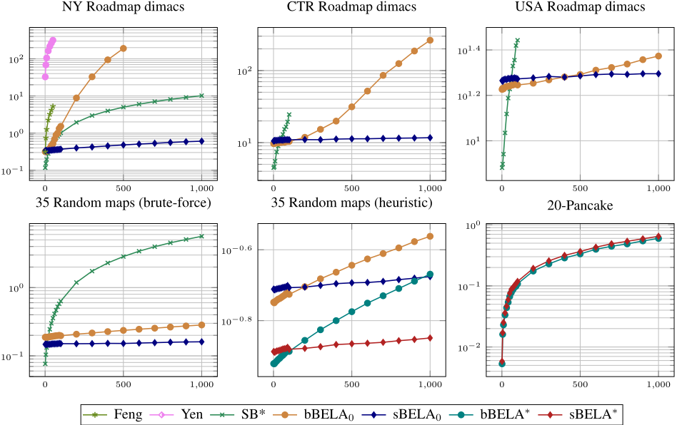
The difference between bBELA0 and sBELA0 is also interesting. The case for bBELA0 could not be more favourable: it only has to expand one centroid, and then to return immediately all paths found since they are all simple. However, it is slower than sBELA0 and the difference increases as k gets larger. As conjectured in Section 4, even if the density of simple solution paths is very large, the length of the solution paths matter. The larger the path, the longer it takes for bBELA0 to verify it is simple, while sBELA0 never does this verification explicitly and thus, it becomes faster.

6.2 Heuristic Search

The purpose of this section is simply to demonstrate that the benefits observed in the brute-force case also translate to heuristic search when solving more difficult instances.

Random maps. The Manhattan distance was used to solve the same instances considered with the brute-force variants. Figure 2 shows the results in this domain. sBELA∗ outperforms bBELA∗ and the difference increases noticeably with larger values of k. The performance of the brute-force variants, bBELA0 and sBELA0 proves the benefits of using heuristics in this domain. As shown, both heuristic variants clearly outperform their brute-force counterparts. Moreover, bBELA∗ is eventually slower than sBELA0 with k = 1 000. 20-Pancake. The 20-Pancake has 2.43 × 1018 nodes, so it was not possible to adapt SB* to solving instances in this domain because they would have not fit in memory. The GAP heuristic [Helmert, 2010] was used for solving 100 randomly generated instances. Figure 2 shows that bBELA∗ is slightly faster than sBELA∗ -less than 0.05 seconds for each value of k. The reason is that the vast majority of paths found are simple and, unlike in the RandomMaps, they are very short, providing bBELA∗ a unique opportunity to find k simple paths very quickly as conjectured in Section 4. The fact that sBELA∗ performs so closely to bBELA∗ in such a favourable case for bBELA∗ is read as a proof of the good performance of sBELA∗ . Indeed, bBELA∗ provides here a baseline that seems very difficult to outperform.

7 Conclusions

The state-of-the-art for solving the k simple shortest-path problem uses the notion of sidetrack edges, and conducts several searches for solving the task. In this paper, it is shown that a much simpler algorithm is possible using the notion of centroids. At the core of its performance is the observation that a simple centroid delivers an arbitrary number of simple paths and that it only conducts a single search. Experiments in different domains show a significant improvement on runtime, while using much less memory.

Acknowledgements

We thank David Coudert for making his source code publicly available and for addressing our questions.

This work was partially funded by grant PID2021127647NB-C21 from MICIU/AEI/10.13039/501100011033, by the ERDF "A way of making Europe", and by the Madrid Government under the Multiannual Agreement with UC3M in the line of Excellence of University Professors (EPUC3M17) in the context of the V PRICIT (Regional Programme of Research and Technological Innovation).