
Online Goal Recognition Using Path Signature and Dynamic Time Warping
Proceedings of the Thirty-Fifth International Joint Conference on Artificial Intelligence. Main Track. Pages 6199-6207.
https://doi.org/10.24963/ijcai.2026/690
© 2026 International Joint Conferences on Artificial Intelligence
Keywords
- Planning and Scheduling: Activity and plan recognition
- Planning and Scheduling: Applications
Abstract
Online goal recognition in continuous domains poses two central challenges: efficiently encoding large trajectories and effectively comparing them.
Recent work addresses these challenges by using custom state-space representations and metrics to compare observations against hypotheses.
However, these approaches often overlook well-established encoding techniques used in other domains that offer substantial advantages.
This paper introduces a novel method for online goal recognition that leverages path signatures, a compact, expressive representation of rough path theory that captures key semantic features of trajectories in an efficient way, enabling more meaningful comparisons between them.
Experiments show that our method consistently outperforms the state of the art in predictive accuracy and online planning efficiency, while remaining competitive offline.
- [Amado and Meneguzzi, 2020] Leonardo Amado and Felipe Meneguzzi. Latrec -recognizing goals in latent space (stu- dent abstract). In Proceedings of the 34th AAAI Confer- ence on Artificial Intelligence, 2020.
- [Amado et al., 2019] Leonardo Amado, João Paulo Aires, Ramon F Pereira, Maurício C Magnaguagno, Roger Granada, Gabriel Paludo Licks, and Felipe Meneguzzi. Latrec: Recognizing goals in latent space (demo). In 29th International Conference on Automated Planning and Scheduling (ICAPS). AAAI Press, 2019.
- [Amado et al., 2022] Leonardo Amado, Reuth Mirsky, and Felipe Meneguzzi. Goal recognition as reinforcement learning. In Thirty-Sixth AAAI Conference on Artificial Intelligence, pages 9644-9651. AAAI Press, 2022.
- [Amado et al., 2023] Leonardo R. Amado, Ramon F. Pereira, and Felipe Meneguzzi. Robust Neuro-Symbolic Goal and Plan Recognition. In Proceedings of the AAAI Conference on Artificial Intelligence. AAAI Press, 2023.
- [Asai and Fukunaga, 2018] Masataro Asai and Alex Fuku- naga. Classical planning in deep latent space: Bridging the subsymbolic-symbolic boundary. In Proceedings of the aaai conference on artificial intelligence, volume 32, 2018.
- [Berndt and Clifford, 1994] Donald J Berndt and James Clif- ford. Using dynamic time warping to find patterns in time series. In Proceedings of the 3rd international conference on knowledge discovery and data mining, pages 359-370, 1994.
- [de A. Santos et al., 2021] Luísa R. de A. Santos, Felipe Meneguzzi, Ramon F. Pereira, and André Pereira. An LP-Based Approach for Goal Recognition as Planning. In Proceedings of the 35th AAAI Conference on Artificial In- telligence (AAAI). AAAI Press, 2021.
- [Elhadad et al., 2026] Osher Elhadad, Felipe Meneguzzi, and Reuth Mirsky. GRAIL: Goal Recognition Alignment through Imitation Learning. In 25th International Confer- ence on Autonomous Agents and Multiagent Systems (AA- MAS). IFAAMAS, 2026.
- [Fang et al., 2023] Zihao Fang, Dejun Chen, Yunxiu Zeng, Tao Wang, and Kai Xu. Real-time online goal recogni- tion in continuous domains via deep reinforcement learn- ing. Entropy, 25(10):1415, 2023.
- [Fikes and Nilsson, 1971] Richard E Fikes and Nils J Nils- son. STRIPS: A new approach to the application of the- orem proving to problem solving. Artificial intelligence, 2(3-4):189-208, 1971. IJCAI
- [Fitzpatrick et al., 2021] Grady Fitzpatrick, Nir Lipovetzky, Michael Papasimeon, Miquel Ramirez, and Mor Vered. Behaviour recognition with kinodynamic planning over continuous domains. Frontiers in Artificial Intelligence, 4, 2021.
- [Gavenski et al., 2024] Nathan Gavenski, Juarez Monteiro, Felipe Meneguzzi, Michael Luck, and Odinaldo Ro- drigues. Explorative imitation learning: A path signature approach for continuous environments. In 27th European Conference on Artificial Intelligence, volume 392, pages 1551-1558, 2024.
- [Jain et al., 2021] Avik Jain, Lawrence Chan, Daniel S Brown, and Anca D Dragan. Optimal cost design for model predictive control. In Learning for Dynamics and Control, pages 1205-1217. Proceedings of Machine Learning Research, 2021.
- [Kaminka et al., 2018a] Gal A Kaminka, Mor Vered, and Noa Agmon. Plan recognition in continuous domains. In AAAI Conference on Artificial Intelligence, 2018.
- [Kaminka et al., 2018b] Gal A Kaminka, Mor Vered, and Noa Agmon. Plan recognition in continuous domains. In Twenty-Seventh AAAI Conference on Artificial Intelli- gence, 2018.
- [Lyons, 1998] Terry J Lyons. Differential equations driven by rough signals. Revista Matemática Iberoamericana, 14(2):215-310, 1998.
- [Masters and Sardina, 2017] Peta Masters and Sebastian Sardina. Cost-based goal recognition for path-planning. In Sixteenth Conference on Autonomous Agents and Mul- tiAgent Systems, pages 750-758, 2017.
- [Meneguzzi and Pereira, 2021] Felipe Meneguzzi and Ra- mon Pereira. A survey on goal recognition as planning. In Thirtieth AAAI Conference on Artificial Intelligence, 2021.
- [Pereira et al., 2019] Ramon Pereira, Nir Oren, and Felipe Meneguzzi. Landmark-based approaches for goal recog- nition as planning. Artificial Intelligence, 279:103217, 12 2019.
- [Ramırez and Geffner, 2009] Miquel Ramırez and Hector Geffner. Plan recognition as planning. In Twenty-First International Joint Conference on Artificial Intelligence, pages 1778-1783. Citeseer, 2009. IJCAI
- [Ramírez and Geffner, 2010] Miguel Ramírez and Hector Geffner. Probabilistic plan recognition using off-the-shelf classical planners. In Twenty-Fourth AAAI Conference on Artificial Intelligence, 2010.
- [Salvador and Chan, 2007] Stan Salvador and Philip Chan. Toward accurate dynamic time warping in linear time and space. Intelligent data analysis, 11(5):561-580, 2007.
- [Serina et al., 2025] Lorenzo Serina, Mattia Chiari, Al- fonso Emilio Gerevini, Luca Putelli, and Ivan Serina. To- wards efficient online goal recognition through deep learn- ing. In Proceedings of the 24th International Conference on Autonomous Agents and Multiagent Systems, pages 1895-1903. International Foundation for Autonomous Agents and Multiagent Systems, 2025.
- [Slotine et al., 1991] Jean-Jacques E Slotine, Weiping Li, et al. Applied nonlinear control, volume 199. Prentice hall Englewood Cliffs, NJ, 1991.
- [Sohrabi et al., 2016] Shirin Sohrabi, Anton V Riabov, and Octavian Udrea. Plan recognition as planning revisited. In Twenty-Fifth International Joint Conference on Artificial Intelligence, pages 3258-3264, 2016. IJCAI
- [Speck et al., 2020] David Speck, Robert Mattmüller, and Bernhard Nebel. Symbolic top-k planning. In Thirty- Fourth AAAI Conference on Artificial Intelligence, pages 9967-9974, 2020.
- [Sturtevant, 2012] Nathan R Sturtevant. Benchmarks for grid-based pathfinding. IEEE Transactions on Computa- tional Intelligence and AI in Games, 4(2):144-148, 2012.
- [Sukthankar et al., 2014] Gita Sukthankar, Christopher Geib, Hung Hai Bui, David Pynadath, and Robert P Goldman. Plan, activity, and intent recognition: Theory and practice. Elsevier, 2014.
- [Tao et al., 2021] Yaguang Tao, Alan Both, Rodrigo I Sil- veira, Kevin Buchin, Stef Sijben, Ross S Purves, Patrick Laube, Dongliang Peng, Kevin Toohey, and Matt Duck- ham. A comparative analysis of trajectory similarity mea- sures. GIScience & Remote Sensing, 58(5):643-669, 2021.
- [Tesch et al., 2024] Douglas Tesch, Leonardo Rosa Amado, and Felipe Meneguzzi. Real-time goal recognition us- ing approximations in euclidean space. In 27th European Conference on Artificial Intelligence, volume 392, pages 3589-3596, 2024.
- [Vered and Kaminka, 2017] Mor Vered and Gal A Kaminka. Heuristic online goal recognition in continuous domains. In Twenty-Sixth AAAI Conference on Artificial Intelli- gence, pages 4447-4454, 2017. IJCAI
- [Vered et al., 2018] Mor Vered, Ramon Fraga Pereira, Gal Kaminka, and Felipe Meneguzzi. Towards online goal recognition combining goal mirroring and landmarks. In Seventeenth International Conference on Autonomous Agents and MultiAgent Systems, pages 10-15, 2018.
- [Wen and Amado, 2025] Jiaqi Wen and Leonardo Amado. Goal recognition via variational causality. In Proceed- ings of the 24th International Conference on Autonomous Agents and Multiagent Systems, pages 2162-2170. Inter- national Foundation for Autonomous Agents and Multia- gent Systems, 2025.
References were extracted automatically from the PDF and may contain errors.
Full text extracted automatically from the PDF; figures, tables and equations may differ. The PDF is the version of record.
1 Introduction
Goal recognition aims to infer the goal of an agent solely based on sparse observations along with knowledge of the environment [Sukthankar et al., 2014]. While research on goal recognition focuses on environments with discrete representations [Meneguzzi and Pereira, 2021], continuous online goal recognition [Kaminka et al., 2018a] aims to support real-time inference in continuous domains while maintaining reliable goal inference. Such approaches often compute the probability of each possible goal by building complete plans that conform to observations as they become available. However, these methods require multiple planner calls that scale linearly with the number of goals and observations [Kaminka et al., 2018b], resulting in substantial computational overhead. This overhead is impractical in applications that require fast results. Recent approaches focus on reducing the computational cost. Vered and Kaminka [2017] used a geometric heuristic to cut unfeasible goals, whereas Tesch et al. [2024] used a light approximation of the complete trajectories to avoid real-time (online) plan computation.
The current trend in goal recognition research in continuous domains focuses on inferring goals directly from the environment's state-space [Kaminka et al., 2018b; Fitzpatrick et al., 2021; Tesch et al., 2024]. These approaches often rely on raw state information (e.g., position, velocity, acceleration, and relative distances), which may not capture the underlying behavioral patterns necessary for robust goal inference. Existing state encodings [Slotine et al., 1991] often fail to capture the temporal structures or semantics of an agent's trajectory (information that is often critical for distinguishing among goals). We address this gap by using path signature [Lyons, 1998] representations. Path signatures encode key semantic characteristics of arbitrarily sized sequences of data, such as agents' trajectories, into unique, fixed-length arrays. They yield compact representations that are invariant to reparametrization and naturally capture multi-scale dependencies, enabling more meaningful comparison between trajectories of varying lengths [Gavenski et al., 2024].
Identifying trajectory differences is also a challenging task for goal recognition [Tao et al., 2021]. These difficulties become especially pronounced in robotic applications, where agents are fast moving [Fitzpatrick et al., 2021]. One possible approach is to use similarity measures tailored to noise, varying path lengths, and non-Euclidean distances. Goal recognition approaches often overlook these measures, despite their close affinity with goal recognition problems. We overcome this challenge by pairing path signatures with Dynamic Time Warping (DTW) [Berndt and Clifford, 1994].
This paper develops Goal Recognition with Path Signatures (GRPS), an approach that leverages path signatures to encode geometric and temporal properties of agents' trajectories. GRPS can be integrated with DTW to provide enhanced predictive performance in settings with noisy or incomplete observations. Our contributions are: (i) an online goal recognition approach using path signatures; and (ii) an enhanced inference step using DTW that further improves predictive accuracy, albeit at an increased inference time. GRPS works in continuous and discrete domains, achieving state-of-the-art results in the former and remaining competitive in the latter.
2 Background
OnlineGoal Recognition We adopt and generalise the goal recognition problem definition of Meneguzzi and Pereira, [2021] to accommodate both continuous and discrete domains. A goal recognition problem F is a tuple ⟨D, G, I, O⟩ with the following elements. The domain D comprises the state space S, the action space A, the observation space O, a transition function T, and a projection function f. States st ∈ S are vectors describing the domain at time t, and can be continuous or discrete. Similarly, actions a ∈ A are vectors that can be continuous or discrete. A transition function T defines how actions transform the environment and need not be Markovian, but in these cases T : S × A → S. A projection function f : S → O maps an underlying state into an observation ot ∈ O. The sequence of observations O then contains state information projected by f. Thus, an observation sequence is a finite sequence of state projections O = [f(s0), · · · , f(sn)], where s0 = I and sn ∈ G. The set of goal hypotheses G ⊂ S enumerates the potential goals of the observed agent, with each goal hypothesis g ∈ G being the final state after a successful plan.
A solution to F is a probability distribution PG over the goal hypotheses G explaining the observations. Similarly, the initial state I ∈ S defines the starting state. In discrete goal recognition problems, the state space S is finite and is often described using STRIPS-style Planning Domain Definition Language (PDDL) representations [Fikes and Nilsson, 1971]. In contrast, in continuous goal recognition problems, the state space lies in the infinite set of real-valued vectors, i.e., Rn . To ensure feasibility within our problem formulation, we require a transformation of states in discrete (STRIPS-style) goal recognition problems into a vectorial representation. We address this conversion in Sec. 4.2. To extend the classic definition to online problems, one must only consider that any given sequence of observations O may not be complete O0:t since the agent is still interacting with the environment.
Early goal recognition methods assume that agents act optimally, following least-cost paths toward their goal [Ramırez and Geffner, 2009]. Under this assumption, goal hypotheses can be ranked by comparing the cost of optimal plans with observed behavior [Ram´ırez and Geffner, 2010; Masters and Sardina, 2017]. Specifically, Ram´ırez and Geffner [2010] compute goal probabilities from the difference in plan costs between plans that must explain the observations and unconstrained optimal plans reaching the same goal. However, these plan-based approaches require repeated calls to a planner, i.e., one for each goal hypothesis and often for each new observation, making them computationally expensive. To reduce computational costs, recent work reasons over precomputed trajectories (state sequences from I to goals) rather than invoking a planner for each new observation [Vered and Kaminka, 2017; Vered et al., 2018; Masters and Sardina, 2017; Tesch et al., 2024]. The resulting path-based goal recognition problem R = ⟨S,G, I, T ,O⟩ has an implicit (and potentially infinite) set of all possible trajectories T from I to G. However, comparing observation sequences against trajectories remains challenging, as trajectories may differ in length, observations may be partial (or noisy), and different state representations may emphasize different structural properties.
Path Signatures Path Signatures [Lyons, 1998] are fixedlength feature vectors that represent multidimensional time series (i.e., trajectories). To compute a path signature β1:n, where n ∈ N, we take a trajectory τ of length belonging to {1, . . . , n}, where each state is a vector in Rd with dimensions indexed by a collection of indices i1, . . . , ik ∈ {1, . . . , d}. For example, in the Moving-AI [Sturtevant, 2012] dataset, each trajectory consists of n states from one point to another, and each state has 3 dimensions. Thus, the recursively computed path signature PS for the trajectory τ for any k ≥ 1 and time t (1 ≤ t ≤ n) as:
Therefore, the signature β of a trajectory τ : [1, n] → Rd is the collection of all the iterated integrals of τ:
where the first term is conventionally 1, and k defines the kth level of the signature, which defines the finite collection of all terms PS(τ)i1,··· ,ik 1:n for the multi-index of length k. For example, when k=d, the last termwould be PS(τ)d,d,··· ,d 1:n .
Finally, path signatures are unique: no two path signatures are equal unless the trajectories that generate them are identical. By leveraging this property, it is possible to construct a trajectory tree TT that encodes a set of all trajectories T by storing all partial path signatures along each branch. The value for the jth node of branch i in the tree corresponds to the path signature of the first j steps of trajectory τ i ∈ T , defined by TTi,j = β(τ i1:j ), where 1 ≤ i ≤ |T |, and 1 ≤ j ≤ |τ i |. This property is useful in our setting because it guarantees a one-to-one correspondence between trajectory prefixes and their encoded signatures, enabling efficient and unambiguous representation of the trajectory space. The supplement 1 explains path signatures in further detail.
Dynamic Time Warping [Berndt and Clifford, 1994] aligns two trajectories by stretching or compressing them in the time dimension to find the best match, i.e., the timestamps with the minimum distance between the trajectories. Berndt and Clifford provide a formal definition of DTW in their work: given two trajectories τ = [s1, s2, · · · , sn] and τ ′ = [s′1 , s′2 , · · · , s′m], the algorithm creates a cost matrix n × m between each pair of sample trajectories si and s′j . Then, with all matrix costs computed, the algorithm searches for a minimum-cost path that links the lower-left and upperright corner elements. Fig. 1 shows the cost matrix between trajectories τ and τ ′ considering the squared Euclidean distance (||si - s′j ||2 ). Note that the orange cells represent the sequence with the minimum cost (27). The output of the DTW algorithm is a vector combining the indices of the elements that best align the sequences. Thus, the output is δ = [(1, 1) ; (2, 2) ; (3, 3) ; (3, 4)], knows as warping path.
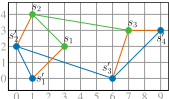
0 1 2 3 4 5 6 7 8 9
| s′1 | s′2 | s′3 | s′4 | |
| s3 | 45 | 50 | 10 | 4 |
| s2 | 16 | 5 | 41 | 65 |
| s1 | 8 | 9 | 13 | 37 |
1 Available at: https://arxiv.org/abs/2605.07736
Squared Distances
Algorithm 1 Goal Recognition with PS and DTW
Require: D,G, I from goal recognition problem
Require: K number of top trajectories
Require: MT , PT , k to build trajectory tree
Goal Recognition with Path Signatures
▷ Offline
- 1: ˆ T ← [ ˆ Tg ↦→ SAMPLEKTRAJ(D, I, g,K) | g ∈ G]
2: TT ← TRAJECTORYTREE( ˆ
T ,MT , PT , k) ▷ Algorithm 2
Dynamic Time Warping
▷ Online
- 3: O← [ ], βO ← [ ]
- 4: when receives ot and ot /∈ G do
- 5: O←O ∪ ot
6: βO ← βO ∪ β(O)k1:t ▷ Compute observations signature
- 7: PG ← {g ↦→ 0 | g ∈ G}
▷ Initialize probabilities
- 8: for br ∈ TT do
- 9: δ ← DTW (βO, br )
- 10: g ← leaf node of br
- 11: p ← 1 - exp (-1/∥βOt-br j ∥2t,j∈δ )
- 12: PG[g] ← max(p, PG[g])
- 13: broadcast PG
3 Goal Recognition with Path Signatures
GRPS has two key innovations: (i) tree structures from set of trajectories ˆ T based on path signatures, further improved by applying merging and pruning operations to identify relevant states across trajectories; and (ii) integrating DTW as a similarity measure to compare path signatures even when they are not temporally aligned. Alg. 1 provides an overview of GRPS+DTW. Importantly, DTW is optional and can be bypassed when computational efficiency is critical, such as in real-time applications. The offline stage begins by computing the top-K approximate trajectories for each goal hypothesis in the problem. This is analogous to recent planning-based goal and plan recognition approaches [Ram´ırez and Geffner, 2010; Sohrabi et al., 2016]. For that, we use a trajectory sampling function SAMPLEKTRAJ that yields ˆ Tg approximately optimal trajectories, given the domain D, the initial configuration I, a goal g ∈ G and a pre-defined number of trajectories K (Alg. 1, Ln. 1). 2 The algorithm then uses the set ˆ T of all top-K trajectories to all goals G, to build the trajectory tree TT (Alg. 2). TRAJECTORYTREE builds this tree by including all partial trajectories from ˆ T . It performs both merging and pruning operations using predefined merging and pruning thresholds (MT , PT , explained in 3.1) to reduce redundancy.
The online stage of GRPS takes new observations o from the agent at time t and computes the partial path signature β(O)k1:t given the depth k and all observations received up to that moment (Ln. 6). GRPS can recognize goals under partial observability, i.e., O is not complete, so β(O)k1:t may lack the information for some (missing) time steps t. After computing the path signature βO, GRPS compares it to all branches under TT (Ln. 8-12). GRPS can use DTW to align O with the current branch (Ln. 9). We leverage the FastDTW implementation [Salvador and Chan, 2007], which typically produces warping paths whose length is close to max(|βO|, |br|). However, this implementation does not guarantee an exact length, and may exceed this value depending on the signal structure and approximation behavior. When |δ| is greater than max(|βO|, |br|), multiple indices of br may map to a single observation index of βO. In such cases, we select the first occurrence of t in δ. For real-time inference, GRPS can bypass the alignment considering that all t in O align perfectly. Then, it retrieves the branch's goal by looking at the leaf node (Ln. 10), and computes the likelihood of that goal g being the goal of the agent (Ln. 11). Finally, GRPS returns the probability distribution over the goal hypotheses (Ln. 13) from which we can extract the most likely goal up to the current time step. For details about the complexity of our method, please refer to the supplementary material.
2 We omit I for simplicity, as all trajectories share the same initial state, but keep g since it varies across trajectory sets.
3.1 Trajectory Tree, Prune andMerge
We introduce pruning and merging operations on trees of path signatures. By computing path signatures at discretely sampled intervals across multiple trajectories, we obtain a tree rooted at the initial position I, where nodes represent path signatures at each timestep t. As trajectories are added, those sharing states produce identical path signatures until divergence, meaning trajectories with common prefixes share partial path signatures up to their final common point. This enables arranging multiple trajectories in a tree where equal partial trajectories share subtrees. A step-by-step numerical example of trajectory tree construction, including path signature computation at each node and the shared-branch structure arising from the uniqueness property, is provided in the supplementary material (Appendix 2.3-2.5).
However, path signatures differ even with slight path divergence, yielding a trajectory tree with width between |G| and |T |. While this sensitivity is vital in rough path theory, it is problematic for matching semantically equivalent trajectories with minor variations: without intervention, trees may share only their root (see supplementary material for the motivation). To address this, we perform merge and prune operations, enabling node sharing across different trajectories. Ideally, any TT built from distinct top-K trajectories ˆ T achieves width K · |G|, verifiable by counting leaves post-processing.
Alg.2 (Ln.6-10) describes the merge operation, which compares all nodes at the same level sharing the same parent and merges those with Euclidean distance below threshold MT . Merging proceeds by selecting the rightmost node, removing it, assigning its children to the leftmost node, and computing their averaged path signature. This operation eliminates slightly different yet closely related nodes, thus merging semantically similar trajectories. By keeping tree levels thin, merging reduces the number of comparisons during goal recognition. However, MT must be chosen carefully: too high a threshold can reduce tree width below |G|. Therefore, it is vital to ensure at least as many leaves as goals.
The prune operation in Alg.2, Ln.11-14, occurs after all merge operations and reduces tree depth by removing nodes within a Euclidean distance PT of their parent, with the parent inheriting the pruned node's children. Since merge operations preserve level comparisons (all siblings share timestep t), performing operations in reverse order would incorrectly compare different timesteps across trajectories. Pruning elim-
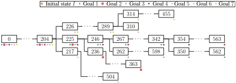
(a) Trajectory tree after merge and prune.
(b) Example landmark (node 204) as the black line.
Figure 2: Example of trajectory tree for the Aftershock map.
inates semantically insignificant observations, e.g., an agent taking many small steps toward a goal, creating nodes that do not alter the trajectory's meaning. Yet, pruning can reduce tree width below |G|, requiring careful selection of PT .
Removing closely related nodes improves efficiency by reducing comparisons with new observations. Goals with similar trajectories correspond to similar branches, reducing redundancy (Fig. 2a). The trajectory tree compactly represents top-K trajectories in continuous space, with nodes analogous to planning landmarks [Pereira et al., 2019]. After merging and pruning, similar goals (Fig. 2b) remain in the same branch until the final bifurcation. For example, goals 4 and 11 share trajectories and split last at node 342.
3.2 Online Goal Recognition with Path Signature
With a fully constructed trajectory tree TT derived from a subset of approximated trajectories ˆ T ⊆ T , GRPS infers the potential goal of an observed agent (see supplementary material for further discussion). We note that to compare the partial path signatures from TT to observations from the agent, either: (i) GRPS has access to the projection function f, allowing it to construct a trajectory tree over observations, i.e., f( ˆ T ); or (ii) observations and states are identical, meaning the projection function is the identity, i.e., f(s) = s.
Initially, GRPS computes the likelihood of a branch br ∈
Algorithm 2 Merge and Prune Operations in Trajectory Tree
Require: ˆ T ,MT and PT resp. merge and prune thresholds Require: k a path signature depth 1: TT ← new trajectory tree with a single node with value 1 2: for each trajectory τ ∈ ˆ T do ▷ Trajectory Tree Creation 3: n← root of TT 4: for t ← 2 . . . |τ | do 5: Add new node c with value β(τ )k1:t as child of n; n ← c 6: for each node n in TT do ▷ Merge Operation 7: for each distinct pair (nz, nj) of children of n do 8: if ∥nβz -nβj ∥2 <MT then 9: Add all of nj's children to nz; Delete nj 10: nβz ← (nβz +nβj )/2 11: for each node n in TT do ▷ Prune Operation 12: for each child node nj of ni do 13: if ∥nβ - nβj ∥2 < PT then 14: Add all of nj 's children to n; Delete nj 15: return Updated trajectory tree TTTT being the current sequence of observations βO:
where ρ is a normalizing term, g is the goal for that branch, and the final term is a prior probability that an agent might choose each goal [Ram´ırez and Geffner, 2010]. This might express a known preference over goals, but is often simply a uniform probability distribution. Here, the probability P(br | g) is always one, since each br can only have one possible goal (leaf), and a uniform prior P(g) avoids biases towards any specific, i.e., all goals are equally likely. Since GRPS does not use DTW, we assume that time steps are perfectly synchronized, i.e., the observed agent's step size is equivalent to the approximated trajectories' step. Therefore, the key part from Eq. 3 is how to compute P(βO | br) since we know all other terms. For this we use Eq. 4, which is similar to equation from Line 11 from Alg. 1.
GRPS remains efficient in iterations of Eq 4 over path signatures by computing the distance between βOt and brt once instead of all o ∈ O as in Fitzpatrick et al..
Rather than averaging probabilities across branches, GRPS uses the maximum likelihood to avoid diluting high probabilities from paths close to the observations with lower probabilities from distant ones. This becomes important when the trajectory tree is built from a large or diverse set of trajectories (as produced by SAMPLEKTRAJ in Alg. 1 Ln. 1), which results in many branches per goal-up to K · |G|. In these cases, averaging probabilities across all branches that lead to the same goal can dilute high-confidence signals, especially when many branches yield low scores due to suboptimal trajectories from I to G. Since path signatures encode rich geometric and temporal structures, even beyond what is captured by the projection function f, their scores can vary substantially between branches.
3.3 Dynamic TimeWarping Integration
Assuming that the sequence of observations O is perfectly synchronized with all trajectories in TT might not be realistic. Therefore, GRPS integrates DTW to solve two main related issues: (i) trajectories and observations that do not share the same characteristics, and (ii) potentially missing time steps from observations. The first issue concerns how the synchronicity assumption in GRPS can be easily violated when trajectories are sampled from agents with different characteristics, such as agents with different velocities or movement patterns from the observed agent (dynamic model error). Since GRPS makes no assumptions about the sampling process, it relies on the information encoded in path signatures to correctly synchronize observations and trajectories. However, merging and pruning also reduce the number of available steps for comparison across each trajectory. Thus, having a function that best aligns indices between one sequence of observations and another sequence of states is crucial for improving performance. The second issue relates to GRPS's online step, which infers a goal only upon receiving a new observation from the agent. Under partial observability, observations may have arbitrary gaps in time, resulting in an incomplete sequence of observations, such as O = [o0, o1, o3], where o2 is missing.
We address the limitation of signature-only comparisons using Dynamic Time Warping (DTW) in Alg. 1 as a similarity measure to better align observations with trajectory branches. This effectively replaces Eq. 4 with Eq. 5.
where δ is the alignment path computed by DTW, consisting of index pairs (i, j) that optimally align each observation index i with a corresponding index j in the trajectory br. However, DTW introduces a non-negligible computational overhead. For each br ∈ TT, DTW has a time complexity of O(|O| · |br|), leading to an overall complexity of O(|TT| · |O| · ⌊TT⌉) (Alg. 1, Ln. 8-12). When combined with the cost of computing path signatures-O(|O| ·dk ) - the resulting inference process becomes relatively expensive for real-time applications. We note that for partial observability settings, GRPS+DTW first interpolate all observations to create an approximated sequence of observations of size t (O1:t). That is, if the initial observations were [I, o2] for t = 2, the approximated observations would be [I, ˆ o1, o2], where ˆ o1 is the interpolated observation. We provide a detailed version of Alg. 1 in the supplementary material.
4 Experiments
We benchmark using accuracy (ACC), the spread of goals in the output (SPR), the number of planner calls (PC) required to infer each goal, Positive Predictive Value (PPV), and the runtime. ACC is the proportion of instances a method infers the goal correctly. SPR is the average number of distinct goals predicted across all instances, indicating how concentrated or diffuse the method's predictions are over the space of goal hypotheses (with a minimum value of 1). PC denotes the number of external planner calls required during inference, serving as a proxy for the computational overhead of planner-based methods. PPV measures the proportion of correctly inferred goals among all inferred predictions, i.e., PPV = TP/TP+FP, where TP and FP denote true and false positives, respectively. Runtime comprises two components: the offline stage, which includes all preprocessing steps, and the online stage, which captures the time required for goal inference per observation sequence.
4.1 Continuous Domains
The experiments use the dataset from Moving-AI [Sturtevant, 2012], which features a simulated yet realistic benchmark comprising 28 scenarios from StarCraft. We select this dataset to ensure a fair comparison between GRPS and previous work, and elaborate on it and how we create trajectories in the supplement. Our experiments use the trajectory sampling procedure from Tesch et al., [2024] as the SAMPLEKTRAJ function. We evaluate both GRPS and GRPS+DTW by varying the trajectory tree parameters, the merge threshold MT , the prune threshold PT , and the number of sampled trajectories per goal K for the sampling function. To identify the most effective parameter combinations, we conduct a grid search across 10 scenarios, ranging threshold values from 0 to 2 in increments of 0.2, and K values in {1, 5, 10, 15}. The experiments use a depth of k = 2 for the path signature, with an ablation provided in the supplement.
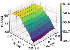
Parameter Search Fig. 3a and 3b show the average PPV among the scenarios for the whole grid search space using K of 1 and 15, respectively. This indicates that the merge variable has a limited influence on recognition process accuracy (rather than efficiency), since the merge process combines similar trajectories. Thus, when the number of trajectories is K = 1, there are no additional trajectories available for merging. By contrast, Figure 3b shows the impact of the merge and prune variables when K = 15, indicating that some level of merging and pruning benefits GRPS, while higher thresholds decrease its performance, which is to be expected. Importantly, it shows that increasing merging has a limited impact on performance, whereas increasing pruning substantially degrades PPV. This suggests that GRPS is more sensitive to reductions in trajectory depth than to reductions in width. In particular, pruning removes deeper prefixes from the trajectory tree, which are often essential for distinguishing between goals, especially when observations are partial or early in the trajectory. On the other hand, merging only collapses similar branches, which tends to preserve overall structure unless applied too aggressively. As a result, while some merging can help reduce redundancy without harming performance, even moderate levels of pruning can lead to underfitting and suppressing informative variations.
Fig. 3c and 3d depict the average grid search results for both inference modes for K = 1 and K = 15. These results show that increasing the prune threshold harms inference quality, as measured by PPV. However, small pruning values in the range of 0.0 to 0.2 offer a distinct advantage by modestly reducing tree depth without significantly harming predictive performance. This balance is especially relevant in online inference, where shallower branches lead to faster traversal and lower computational overhead. Thus, selecting appropriate thresholds is not only a matter of accuracy but also efficiency. Based on these experiments, we adopt pruning and merging values of 0.2 when using GRPS, and 0.6 for pruning and 0.2 for merging when using GRPS+DTW, striking a balance between preserving informative structure and maintaining inference efficiency.
Continuous Results Tab. 1a compares the results of our two inference modes with recent work: Vector [Tesch et al., 2024], Mirroring [Kaminka et al., 2018b], and Recompute plus Prune (R+P) [Vered and Kaminka, 2017]. Tab. 1a shows the average values across all scenarios in the Moving- AI dataset, excluding the 10 scenarios used for ablation. We report the mean of each metric (and its standard deviation) across all experiments (see supplement for details).
| (a) Continuous Domains | (b) Discrete Domains | ||||||||||
|---|---|---|---|---|---|---|---|---|---|---|---|
| Metrics | Mirr. | R+P | Vector | GRPS | + DTW | Mirr. | Land. | GM+L | Vector | GRPS | + DTW |
| PPV (%) | 38.7 ± 7.0 | 42.1 ± 5.7 | 47.9 ± 9.0 | 50.7 ±9.4 | 53.6 ±8.5 | 47.3 ±13.6 | 44.8 ±11.2 | 48.2 ±11.5 | 49.2 ±8.9 | 52.0 ±10.5 | 51.9 ±10.4 |
| ACC (%) | 84.6 ± 1.8 | 85.4 ± 1.4 | 86.4 ± 2.1 | 85.9 ±2.7 | 86.7 ±2.4 | 81.8 ±8.1 | 82.7 ±5.2 | 84.7 ±5.0 | 84.2 ±5.7 | 85.3 ±6.0 | 85.3 ± 6.0 |
| SPR | 1.0 ±0.0 | 1.1 ±0.02 | 1.0 ± 0.0 | 1.0 ±0.0 | 1.0 ±0.0 | 2.5 ±1.2 | 1.6 ±0.51 | 1.3 ±0.47 | 1.7 ±0.44 | 1.6 ±0.47 | 1.6 ±0.47 |
| PC | 49.0 ± 0.0 | 30.1 ± 1.6 | 7.0 ± 0.0 | 7.0 ±0.0 | 7.0 ±0.0 | 124.8 ±57.4 | 0.0 ±0 | 29.9 ±7.9 | 8.2 ±3.9 | 8.2 ±3.9 | 8.2 ± 3.9 |
| Online (s) | 1.2e4 ±6.2e3 | 5.9e3 ±3.2e3 | 3.9e-2 ±7.0e-4 | 3.0e-2 ±2.1e-3 | 20.5 ±6.6 | 80.4 ±117.6 | 5.7e-1 ±6.1e-1 | 12.5 ±12.5 | 6.4e-2 ±1.3e-1 | 10.1 ±27.4 | 97.6 ±253.8 |
| Offline (s) | 2.9e3 ±1.8e3 | 2.8e3 ±1.7e3 | 1.7e2 ±38.8 | 3.3e2 ±70.7 | 2.8e2 ±55.7 | 4.6 ±5.3 | 1.3e-1 ±2.6e-1 | 4.8 ±5.8 | 33.66 ±63.7 | 60.6 ±76.9 | 62.9 ±80.1 |
GRPS+DTW achieves the highest PPV (53.6%) and ACC (86.7%) across all evaluated method, with GRPS closely following at 50.7% PPV and 85.9% ACC, both surpassing the current state-of-the-art (Vector). This improvement in PPV is particularly significant, as it reflects the method's ability to generate correct predictions. Unlike ACC, which is affected by class imbalance and rewards methods that often predict the majority class, PPV penalizes false positives and better reflects precision at early or ambiguous nodes, where goal recognition is most challenging. Notably, GRPS achieves this improvement in PPV while also reducing Online inference time (from 3.9e-2s to 3.0e-2s). Both inference modes maintain perfect prediction focus (SPR = 1.0) and require the fewest planner calls (PC = 7.0), indicating that they remain computationally efficient as predictive quality improves.
These results reinforce the central motivation behind GRPS: the need for more meaningful and coherent comparisons between agent behavior and candidate trajectories in goal recognition tasks. By leveraging path signatures, GRPS
58.0
57.0
56.0
54.9
53.9
60.4
58.8
57.2
55.6
54.0
60.4
58.7
57.1
55.4
53.8
captures rich geometric and temporal dynamics while remaining robust to suboptimal behavior. Importantly, this added expressiveness does not compromise runtime performance; GRPS remains lightweight and fast enough for real-time applications, with an average inference time of just 30ms. Although GRPS incurs slightly higher Offline times, this is primarily due to its use of Vector's sampling function for generating top-K trajectories. This component, while effective, is not intrinsic to our method. For example, adopting a more efficient sampling strategy or using a dataset of past trajectories could reduce the offline cost of GRPS without affecting its inference (further discussed in supplement). Moreover, GRPS+DTW builds upon this strength by introducing dynamic temporal alignment, enabling even more accurate trajectory-observation comparisons. While it incurs a higher online cost (20.5s), the resulting improvements in both PPV and ACC make it ideal for use in offline or high-precision inference settings. Together, both modes offer a versatile framework that adapts to diverse constraints. This dual capability demonstrates that our approach not only advances the state-of-the-art but also provides a practical and generalizable solution to goal recognition.
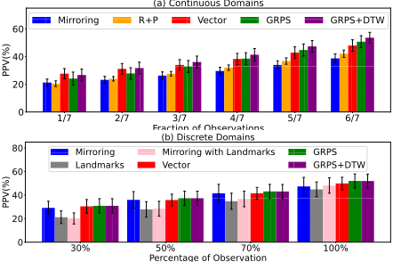
Fig. 4a compares the approaches by their PPV (and its margin of error with a confidence level of 95%), at observation fractions of 1/7 to 6/7 of the full observation length. GRPS is competitive at initial observability stages (1/7, 2/7) and outperforms the other methods at mid-end stages of observability. GRPS+DTW outperforms the other methods at almost all stages of observability, except at the initial stage (1/7), where the available information is insufficient to provide a reliable path signature representation.
4.2 Discrete Domains
The discrete-domain experiments use the goal and plan recognition dataset [de A. Santos et al., 2021]. We select this dataset to ensure a fair comparison with previous work. The dataset comprises thousands of goal-recognition problems across large, non-trivial planning instances in the STRIPS fragment of PDDL. It incorporates domains and problems from established benchmark datasets, including those proposed by Ramırez and Geffner, [2009]. Tab. 1b compares our two inference methods with recent work on goal recognition: Vector [Tesch et al., 2024], Mirroring [Kaminka et al., 2018b], and Goal Recognition with Landmarks and Goal Mirroring with Landmarks both from Vered et al., [2018]. We
PPV(%)
PPV(%)
58
57
56
55
54
0.0 0.5 1.0
Prune
2.0
2.0
0.5
0.0
Merge
(a) GRPS with K = 1.
60
58
56
54
0.0 0.5 1.0
Prune
2.0
2.0
0.5
0.0
Merge
(c) Average for GRPS.
60
58
56
54
0.0 0.5 1.0
Prune
2.0
2.0
0.5
0.0
Merge
(b) GRPS with K = 15.
(d) Average for GRPS+DTW.
Figure 3: Grid search results.
1.5
1.5
1.5
1.5
1.0
1.0
PPV(%)
1.5
1.5
1.0
use SymK [Speck et al., 2020] as the sampler.
There are two important details to consider when applying our goal recognition formulation to discrete-domain problems. First, a direct implementation in discrete STRIPS environments is infeasible, as our formulation assumes vectorand numeric-based representations rather than symbolic descriptions. To overcome this limitation, we use a vectorization of the STRIPS representation [Asai and Fukunaga, 2018], that encode states as fixed-size binary vectors over the complete grounding of predicates. Second, our experiments show that binary vector representations are insufficient to discriminate among trajectories. This limitation persists even when enhanced with signature representation. In the absence of a more meaningful vector representation, we diminish this problem by changing the Ln. 12 of Alg. 1 to PG[g] ← PG[g] + p-PG[g] ng+1 , ng ← ng + 1, where ng is a counter to keep in track the incremental mean computation. The mean of the Top-k signatures favors the hypothesis with the greatest number of similarities to the observations.
We follow the same empirical grid search presented in Sec. 4 on 5 of 12 environments to find optimal merge and prune thresholds. In it, we observe that the best values for merge and prune remain zero (see supplementary material for full ablation test results). Unlike continuous environments, results for the discrete environments deteriorated as values exceeded 0. We hypothesize that this behavior comes from the fact that path signatures use geometrical information to semantically encode different trajectories. Yet, discrete environments states are either: (i) encode information in a non-geometrical manner (e.g., one-hot encoding where values represent categorical states without any inherent spatial or geometric relationships), or (ii) represent transitions that are abrupt and lack continuity, making it difficult for path signatures to capture meaningful patterns. Consequently, path signatures in discrete spaces produce highly dissimilar representations for each state transition, reducing the effectiveness of pruning operations. Furthermore, discrete state spaces are finite, which increases the probability of shared trajectory prefixes, limiting the constraint on possible paths and, thus, reducing merging operations.
Nevertheless, the performance reported in Tab. 1b is competitive with other goal recognition approaches in discrete settings, underscoring the robustness and versatility of GRPS. Fig. 4b compares the approaches by their PPV (and its margin of error with a confidence level of 95%), at 30%, 50%, 70%, and 100% of their respective full observation. Unlike the continuous relative, GRPS and GRPS +DTW slightly outperform other methods across all stages of observability. However, the differences between both are not statistically significant, given the previously mentioned vectorization issues.
5 RelatedWork
Recent approaches to online goal recognition infer goals by measuring the error between a reference trajectory and the observed state using Euclidean distance. Fitzpatrick et al. extend the previous state-of-the-art [Kaminka et al., 2018b], which relies on consecutive planner calls for each new observation in a scenario while ignoring obstacles. Such approaches are unsuitable for real-time applications since relying on calls to a planner incurs an unacceptable computational cost [Jain et al., 2021]. Tesch et al. show that a representative number of suboptimal trajectories is sufficient to perform goal inference without relying on consecutive planner call at each observation. Amado et al.; Amado and Meneguzzi; Amado et al.; Fang et al.; Amado et al.; Wen and Amado; Serina et al.; Elhadad et al., [2019; 2020; 2023; 2023; 2022; 2025; 2025; 2026] leverage machine learning to avoid using planner calls, allowing real-time inference. Unlike our approach, they require pre-existing datasets to train the model.
6 Conclusion
In this paper, we introduced GRPS, a novel data-driven framework for recognizing goals from observation sequences. Unlike traditional approaches, GRPS does not rely on optimality assumptions or costly planner interactions. It leverages path signatures, a compact and expressive representation of trajectories, to compare observed behavior against sampled trajectories in a principled and efficient way.
Extensive evaluation on standard benchmarks shows that GRPS outperforms existing state-of-the-art methods in both precision and planning efficiency, while maintaining strong generalization across scenarios and parameter settings. While better sampling strategies can be easily incorporated to improve recognition accuracy, key future work consists of developing more efficient ways to find the merge and prune hyperparameters. Similarly, improvement in discrete domains requires better vector encoding techniques.
GRPS assumes access to accurate projection functions for trajectory comparison. In real-world settings, where noise or high dimensional observations (e.g., raw sensor data or images) are more prevalent, dynamic time warping becomes necessary. GRPS+DTW does achieve state-of-the-art accuracy, but DTW's added computational cost limits its applicability. In future work, we plan to explore approximate or differentiable variants of DTW that preserve alignment quality while reducing runtime, making it more accessible for realtime goal recognition.
Contribution Statement
Douglas Tesch and Nathan Gavenski have contributed equally to this work.
Acknowledgments
This work was partially supported by UK Research and Innovation [grant number EP/S023356/1], in the UKRI Centre for Doctoral Training in Safe and Trusted Artificial Intelligence (www.safeandtrustedai.org).
This study was financed in part by the Coordenac¸˜ao de Aperfeic¸oamento de Pessoal de N´ıvel Superior Brasil (CAPES) - Finance Code 001.
@inproceedings{ijcai2026p690,
  title     = {Online Goal Recognition Using Path Signature and Dynamic Time Warping},
  author    = {Tesch, Douglas and Gavenski, Nathan and Rosa Amado, Leonardo and Rodrigues, Odinaldo and Meneguzzi, Felipe},
  booktitle = {Proceedings of the Thirty-Fifth International Joint Conference on
               Artificial Intelligence, {IJCAI-26}},
  publisher = {International Joint Conferences on Artificial Intelligence Organization},
  editor    = {Diego Calvanese},
  pages     = {6199--6207},
  year      = {2026},
  month     = {8},
  note      = {Main Track},
  doi       = {10.24963/ijcai.2026/690},
  url       = {https://doi.org/10.24963/ijcai.2026/690},
}
TY - CPAPER TI - Online Goal Recognition Using Path Signature and Dynamic Time Warping AU - Tesch, Douglas AU - Gavenski, Nathan AU - Rosa Amado, Leonardo AU - Rodrigues, Odinaldo AU - Meneguzzi, Felipe T2 - Proceedings of the Thirty-Fifth International Joint Conference on Artificial Intelligence, IJCAI-26 PB - International Joint Conferences on Artificial Intelligence Organization PY - 2026 SP - 6199 EP - 6207 DO - 10.24963/ijcai.2026/690 UR - https://doi.org/10.24963/ijcai.2026/690 ER -Copied
Machine-readable versions of this paper, for tools and AI agents:





