
Unifying Perspectives: Plausible Counterfactual Explanations on Global, Group-wise, and Local Levels
Proceedings of the Thirty-Fifth International Joint Conference on Artificial Intelligence. Main Track. Pages 571-579.
https://doi.org/10.24963/ijcai.2026/65
Keywords
- Machine Learning: Explainable/Interpretable machine learning
- AI Ethics, Trust, Fairnes: Explainability and interpretability
- Machine Learning: Classification
- Machine Learning: Other
Abstract
The growing complexity of AI systems has intensified the need for transparency through Explainable AI (XAI). Counterfactual explanations (CFs) offer actionable "what-if" scenarios on three levels: Local CFs providing instance-specific insights, Global CFs addressing broader trends, and Group-wise CFs (GWCFs) striking a balance and revealing patterns within cohesive groups. Despite the availability of methods for each granularity level, the field lacks a unified method that integrates these complementary approaches. We address this limitation by proposing a gradient-based optimization method for differentiable models that generates Local, Global, and Group-wise Counterfactual Explanations in a unified manner. We especially enhance GWCF generation by combining instance grouping and counterfactual generation into a single efficient process, replacing traditional two-step methods. Moreover, to ensure trustworthiness, we innovatively introduce the integration of plausibility criteria into the GWCF domain, making explanations both valid and realistic. Our results demonstrate the method's effectiveness in balancing validity, proximity, and plausibility while optimizing group granularity, with practical utility validated through practical use cases.
- [Adadi and Berrada, 2018] Amina Adadi and Mohammed Berrada. Peeking inside the black-box: A survey on explainable artificial intelligence (XAI). IEEE Access, 6:52138-52160, 2018.
- [Aeberhard and Forina, 1992] Stefan Aeberhard and M. Fo- rina. Wine. UCI Machine Learning Repository, 1992. DOI: https://doi.org/10.24432/C5PC7J. DOI
- [Alpaydin and Kaynak, 1998] E. Alpaydin and C. Kay- nak. Optical Recognition of Handwritten Digits. UCI Machine Learning Repository, 1998. DOI: https://doi.org/10.24432/C50P49. DOI
- [Artelt and Gregoriades, 2024] André Artelt and Andreas Gregoriades. A two-stage algorithm for cost-efficient multi-instance counterfactual explanations. In Luca Longo, Weiru Liu, and Grégoire Montavon, editors, 2nd World Conference on eXplainable Artificial Intelligence (xAI-2024), Valletta, Malta, July 17-19, volume 3793 of CEUR Workshop Proceedings, pages 233-240, 2024.
- [Artelt and Hammer, 2020] André Artelt and Barbara Ham- mer. Convex density constraints for computing plausible counterfactual explanations. In Artificial Neural Networks and Machine Learning -ICANN 2020 -29th International Conference on Artificial Neural Networks, Bratislava, Slo- vakia, September 15-18, 2020, Proceedings, Part I, vol- ume 12396 of Lecture Notes in Computer Science, pages 353-365. Springer, 2020.
- [Bewley et al., 2024] Tom Bewley, Salim I. Amoukou, Saumitra Mishra, Daniele Magazzeni, and Manuela Veloso. Counterfactual metarules for local and global re- course. In Forty-first International Conference on Machine Learning, ICML 2024, Vienna, Austria, July 21-27, 2024. OpenReview.net, 2024.
- [Carrizosa et al., 2024] Emilio Carrizosa, Jasone Ramírez- Ayerbe, and Dolores Romero Morales. Mathematical opti- mization modelling for group counterfactual explanations. European Journal of Operational Research, 319(2):399- 412, 2024.
- [Dhurandhar et al., 2018] Amit Dhurandhar, Pin-Yu Chen, Ronny Luss, Chun-Chen Tu, Pai-Shun Ting, Karthikeyan Shanmugam, and Payel Das. Explanations based on the missing: Towards contrastive explanations with pertinent negatives. In Advances in Neural Information Processing Systems 31, NeurIPS 2018, pages 590-601, 2018.
- [Dinh et al., 2015] Laurent Dinh, David Krueger, and Yoshua Bengio. NICE: non-linear independent compo- nents estimation. In 3rd International Conference on Learning Representations, ICLR 2015, San Diego, CA, USA, May 7-9, 2015, Workshop Track Proceedings, 2015.
- [Dinh et al., 2017] Laurent Dinh, Jascha Sohl-Dickstein, and Samy Bengio. Density estimation using real NVP. In 5th International Conference on Learning Representations, ICLR 2017, Toulon, France, April 24-26, 2017, Confer- ence Track Proceedings, 2017. [FICO, 2018] FICO. FICO (HELOC) Dataset. https://www.kaggle.com/datasets/averkiyoliabev/ home-equity-line-of-creditheloc, 2018. Accessed: 2026-01-05. Link
- [Fragkathoulas et al., 2024] Christos Fragkathoulas, Vasiliki Papanikou, Evaggelia Pitoura, and Evimaria Terzi. Fgce: Feasible group counterfactual explanations for auditing fairness, 2024.
- [Goodman and Flaxman, 2017] Bryce Goodman and Seth R. Flaxman. European union regulations on algorithmic decision-making and a "right to explanation". AI Mag., 38(3):50-57, 2017.
- [Guidotti, 2022] Riccardo Guidotti. Counterfactual explana- tions and how to find them: literature review and bench- marking. Data Mining and Knowledge Discovery, pages 1-55, 04 2022.
- [Kanamori et al., 2020] Kentaro Kanamori, Takuya Takagi, Ken Kobayashi, and Hiroki Arimura. DACE: distribution- aware counterfactual explanation by mixed-integer linear optimization. In Proceedings of the Twenty-Ninth Inter- national Joint Conference on Artificial Intelligence, IJCAI 2020, pages 2855-2862. ijcai.org, 2020.
- [Kanamori et al., 2022] Kentaro Kanamori, Takuya Takagi, Ken Kobayashi, and Yuichi Ike. Counterfactual explana- tion trees: Transparent and consistent actionable recourse with decision trees. In International Conference on Ar- tificial Intelligence and Statistics, AISTATS 2022, 28-30 March 2022, Virtual Event, volume 151 of Proceedings of Machine Learning Research, pages 1846-1870. PMLR, 2022.
- [Karimi et al., 2022] Amir-Hossein Karimi, Gilles Barthe, Bernhard Schölkopf, and Isabel Valera. A survey of al- gorithmic recourse: Contrastive explanations and conse- quential recommendations. ACM Comput. Surv., 55(5), December 2022.
- [Kavouras et al., 2024] Loukas Kavouras, Eleni Psaroudaki, Konstantinos Tsopelas, Dimitrios Rontogiannis, Nikolaos Theologitis, Dimitris Sacharidis, Giorgos Giannopoulos, Dimitrios Tomaras, Kleopatra Markou, Dimitrios Gunop- ulos, Dimitris Fotakis, and Ioannis Emiris. Glance: Global actions in a nutshell for counterfactual explainabil- ity. arXiv preprint arXiv:2405.18921, 2024.
- [Keane et al., 2021] Mark T. Keane, Eoin M. Kenny, Eoin Delaney, and Barry Smyth. If only we had better coun- terfactual explanations: Five key deficits to rectify in the evaluation of counterfactual XAI techniques. In Proceed- ings of the Thirtieth International Joint Conference on Ar- tificial Intelligence, IJCAI 2021, Virtual Event / Montreal, Canada, 19-27 August 2021, 2021. IJCAI
- [Ley et al., 2022] Dan Ley, Saumitra Mishra, and Daniele Magazzeni. Global counterfactual explanations: Inves- tigations, implementations and improvements. CoRR, abs/2204.06917, 2022.
- [Ley et al., 2023] Dan Ley, Saumitra Mishra, and Daniele Magazzeni. GLOBE-CE: A translation based approach for global counterfactual explanations. In Andreas Krause, Emma Brunskill, Kyunghyun Cho, Barbara Engelhardt, Sivan Sabato, and Jonathan Scarlett, editors, International Conference on Machine Learning, ICML 2023, 23-29 July 2023, Honolulu, Hawaii, USA, volume 202 of Proceed- ings of Machine Learning Research, pages 19315-19342.
- PMLR, 2023.
- [Liu et al., 2012] Fei Tony Liu, Kai Ming Ting, and Zhi-Hua Zhou. Isolation-based anomaly detection. ACM Transac- tions on Knowledge Discovery from Data (TKDD), 6(1):1- 39, 2012.
- [Mahajan et al., 2019] Divyat Mahajan, Chenhao Tan, and Amit Sharma. Preserving causal constraints in counterfac- tual explanations for machine learning classifiers. CoRR, abs/1912.03277, 2019.
- [Martins and Astudillo, 2016] André F. T. Martins and Ramón Fernandez Astudillo. From softmax to sparsemax: A sparse model of attention and multi-label classification. In Proceedings of the 33nd International Conference on Machine Learning, NY, USA, June 19-24, 2016, volume 48 of JMLR Workshop and Conference Proceedings, pages 1614-1623. JMLR.org, 2016.
- [Mothilal et al., 2020] Ramaravind Kommiya Mothilal, Amit Sharma, and Chenhao Tan. Explaining machine learning classifiers through diverse counterfactual ex- planations. In FAT* '20: Conference on Fairness, Accountability, and Transparency, Barcelona, Spain, January 27-30, 2020, pages 607-617. ACM, 2020.
- [Papamakarios et al., 2017] George Papamakarios, Iain Murray, and Theo Pavlakou. Masked autoregressive flow for density estimation. In Advances in Neural Information Processing Systems 30, December 4-9, 2017, Long Beach, CA, USA, pages 2338-2347, 2017.
- [Paszke et al., 2019] Adam Paszke, Sam Gross, Francisco Massa, Adam Lerer, James Bradbury, Gregory Chanan, Trevor Killeen, Zeming Lin, Natalia Gimelshein, Luca Antiga, Alban Desmaison, Andreas Kopf, Edward Yang, Zachary DeVito, Martin Raison, Alykhan Tejani, Sasank Chilamkurthy, Benoit Steiner, Lu Fang, Junjie Bai, and Soumith Chintala. Pytorch: An imperative style, high- performance deep learning library. In Advances in Neu- ral Information Processing Systems 32, pages 8024-8035.
- Curran Associates, Inc., 2019.
- [Pawelczyk et al., 2020] Martin Pawelczyk, Klaus Broele- mann, and Gjergji Kasneci. Learning model-agnostic counterfactual explanations for tabular data. In Proceed- ings of the web conference 2020, pages 3126-3132, 2020.
- [Plumb et al., 2020] Gregory Plumb, Jonathan Terhorst, Sri- ram Sankararaman, and Ameet Talwalkar. Explaining groups of points in low-dimensional representations. In Proceedings of the 37th International Conference on Ma- chine Learning, ICML 2020, 13-18 July 2020, Virtual Event, volume 119 of Proceedings of Machine Learning Research, pages 7762-7771. PMLR, 2020.
- [Ramamurthy et al., 2020] Karthikeyan Natesan Rama- murthy, Bhanukiran Vinzamuri, Yunfeng Zhang, and Amit Dhurandhar. Model agnostic multilevel explana- tions. In Advances in Neural Information Processing Systems 33, NeurIPS, 2020.
- [Rawal and Lakkaraju, 2020] Kaivalya Rawal and Himabindu Lakkaraju. Beyond individualized recourse: Interpretable and interactive summaries of actionable recourses. In Hugo Larochelle, Marc'Aurelio Ranzato, Raia Hadsell, Maria-Florina Balcan, and Hsuan-Tien Lin, editors, Advances in Neural Information Processing Systems 33, 2020.
- [Rezende and Mohamed, 2015] Danilo Rezende and Shakir Mohamed. Variational inference with normalizing flows. In International Conference on Machine Learning, pages 1530-1538. PMLR, 2015.
- [Russell, 2019] Chris Russell. Efficient search for diverse coherent explanations. In Proceedings of the conference on fairness, accountability, and transparency, pages 20- 28, 2019.
- [Samek and Müller, 2019] Wojciech Samek and Klaus- Robert Müller. Towards explainable artificial intelligence. In Explainable AI: Interpreting, Explaining and Visual- izing Deep Learning, volume 11700 of Lecture Notes in Computer Science, pages 5-22. Springer, 2019.
- [Van Rossum and Drake Jr, 1995] Guido Van Rossum and Fred L Drake Jr. Python reference manual. Centrum voor Wiskunde en Informatica Amsterdam, 1995.
- [Wachter et al., 2017] Sandra Wachter, Brent D. Mittelstadt, and Chris Russell. Counterfactual explanations without opening the black box: Automated decisions and the GDPR. CoRR, abs/1711.00399, 2017.
- [Warren et al., 2024] Greta Warren, Eoin Delaney, Christophe Guéret, and Mark T. Keane. Explaining multiple instances counterfactually: User tests of group- counterfactuals for xai. In Case-Based Reasoning Research and Development: 32nd International Con- ference, ICCBR 2024, Merida, Mexico, July 1-4, 2024, Proceedings, page 206-222. Springer-Verlag, 2024.
- [Wielopolski et al., 2024] Patryk Wielopolski, Oleksii Fur- man, Jerzy Stefanowski, and Maciej Zięba. Probabilisti- cally plausible counterfactual explanations with normaliz- ing flows. In ECAI 2024. IOS Press, 2024.
- [Wightman, 1998] Linda F. Wightman. Lsac national longi- tudinal bar passage study. lsac research report series. Tech- nical report, Law School Admission Council, Newtown, PA., 1998.
References were extracted automatically from the PDF and may contain errors.
Full text extracted automatically from the PDF; figures, tables and equations may differ. The PDF is the version of record.
1 Introduction
The increasing complexity of AI systems has fueled regulatory and societal demands for transparency, a need addressed by Explainable AI (XAI) [Goodman and Flaxman, 2017; Wachter et al., 2017; Adadi and Berrada, 2018; Samek and Müller, 2019]. Among XAI techniques, counterfactual explanations (CFs) are particularly valuable for providing actionable "what-if" scenarios that specify how input feature changes can alter model predictions [Wachter et al., 2017]. For example, a CF could show a loan applicant the precise changes needed for loan approval, offering actionable feedback crucial in many fields [Guidotti, 2022]. 1
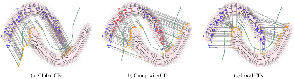
Counterfactual explanations can be generated at three distinct levels of granularity. The most popular Local CFs offer tailored guidance for individual instances but miss broader patterns [Fragkathoulas et al., 2024; Carrizosa et al., 2024]. Global CFs provide high-level summaries for entire datasets but lack individual specificity [Ramamurthy et al., 2020; Plumb et al., 2020]. Bridging this gap, group-wise counterfactual explanations (GWCFs) explain cohesive data subsets, revealing shared patterns while maintaining actionable insights, which is crucial for policy-making in sensitive domains [Carrizosa et al., 2024; Kanamori et al., 2022; Warren et al., 2024]. A detailed comparison of these approaches is illustrated in Figure 1 and discussed in Appendix A.
Despite their promise, existing GWCF methods face significant challenges. Most rely on a two-step process of first clustering data and then generating CFs (or vice versa), which is inefficient and dependent on clustering parameterization [Kavouras et al., 2024; Artelt and Gregoriades, 2024]. Furthermore, ensuring the plausibility of CFs-that is, their alignment with the data distribution and real-world constraints-remains a key challenge, as unrealistic explanations undermine trust and actionability [Artelt and Hammer, 2020].
To address these challenges, we propose a unified framework for generating local, group-wise, and global counterfactuals, as illustrated in Figure 1. Our end-to-end, gradientbased method simultaneously optimizes instance grouping and counterfactual generation, eliminating the inefficient two-step process common in prior work. It can dynamically generate explanations for a varying number of groups, automatically balancing a number through regularization. By formulating this as a single optimization problem, our method efficiently produces CFs at any desired granularity. Crucially, we introduce a probabilistic plausibility criterion, using normalizing flows for density estimation [Rezende and Mohamed, 2015], to ensure that explanations are not only valid but also realistic and actionable.
In summary, our key contributions are:
- A novel unified approach for generating CFs at local,
1 An extended version of this paper with the full appendices is available at https://arxiv.org/abs/2405.17642.
group-wise, and global levels, dynamically adapting to user needs and automatically balancing groups diversity and granularity, leveraging gradient-based optimization.
- A significant advancement in GWCFs generation through end-to-end optimization that unifies group discovery and counterfactual generation while introducing probabilistic plausibility constraints in this domain.
- An experimental evaluation and real-world use case analysis demonstrating our approach's performance, providing the effective balance between validity, proximity, plausibility, and the number of shifting vectors.
2 RelatedWorks
Local Counterfactual Explanations. Local CFs identify minimal feature changes to alter a model's prediction for a single instance [Wachter et al., 2017]. While early methods were often heuristic-based, subsequent work has introduced more sophisticated techniques, including gradient-based optimization, generative models, and contrastive explanations, to improve CF quality and diversity [Dhurandhar et al., 2018; Russell, 2019; Kanamori et al., 2020; Mothilal et al., 2020; Guidotti, 2022]. However, ensuring the plausibility and actionability of these explanations remains an ongoing challenge [Keane et al., 2021].
Global and Group-wise Counterfactual Explanations. Global and group-wise CFs extend explanations beyond single instances to entire datasets or cohesive subgroups. Global approaches seek a single or a few explanations for all instances, using techniques like feature space translations [Plumb et al., 2020], actionable rule sets [Rawal and Lakkaraju, 2020; Ley et al., 2022], or scalable vector-based methods [Ley et al., 2023]. Group-wise methods provide more granular insights. Some approaches partition the input space using tree structures to assign collective actions [Ramamurthy et al., 2020; Kanamori et al., 2022; Bewley et al., 2024]. Others follow a two-step process, first generating local CFs and then clustering them to find group-level explanations [Kavouras et al., 2024; Artelt and Gregoriades, 2024].
These two-step methods, however, can be inefficient and sensitive to clustering parameters.
Plausible Counterfactual Explanations. Plausibility ensures that a CF resides in a high-density region of the data manifold, making it realistic and trustworthy. Various techniques have been proposed to enforce this, such as imposing density constraints using Gaussian Mixture Models [Artelt and Hammer, 2020] or normalizing flows [Wielopolski et al., 2024]. Other approaches leverage causal constraints [Mahajan et al., 2019] or generative models like VAEs to learn the data manifold and generate plausible CFs from it [Pawelczyk et al., 2020]. A comprehensive survey by [Karimi et al., 2022] details the challenges and opportunities in this area.
3 Background
Counterfactual Explanations. Following [Wachter et al., 2017], a local counterfactual explanation finds a new instance x→ → RD for an original instance x0 → RD such that the prediction of a model h changes to a desired class y→ , i.e., h(x→ ) = y→ . The instance x→ is typically found by solving the optimization problem:
The function ε(·↪ ·) refers to a loss function tailored for classification tasks such as the 0-1 loss or cross-entropy. On the other hand, d(·↪ ·) quantifies the distance between the original input x0 and its counterfactual counterpart x→ , employing metrics like the L1 (Manhattan) or L2 (Euclidean) distances to evaluate the deviation. The parameter ω ↑ 0 plays a pivotal role in regulating the trade-off, ensuring that the counterfactual explanation remains sufficiently close to the original instance while altering the prediction outcome as intended.
Plausible Counterfactual Explanations. To ensure realism, [Artelt and Hammer, 2020] introduced a plausibility constraint, requiring the counterfactual x→ to lie in a high-density region of the data distribution p(x♣y→ ) for the target class. The optimization problem becomes:
where p(x→ ♣y→ ) denotes conditional probability of the counterfactual explanation x→ under desired target class value y→ and ϑ represents the density threshold.
Global and Group-wise Counterfactual Explanations. Global and group-wise explanations extend the local concept by applying a shared change vector d to a set of instances. For a global explanation, a single vector d is applied to all instances. For group-wise explanations, different vectors are found for different subgroups of the data. The counterfactual for an instance x0 is then generated by a simple update:
where d is the shift vector of size D, which remains invariant across all observations within the same class or group.
In contrast to the standard formulation, GLOBE-CE [Ley et al., 2023] introduces a scaling factor, k, specific to each observation, allowing for individual adjustments to the magnitude of the shift:
4 Method
4.1 Global Counterfactual Explanations
The base problem of global counterfactual explanation assumes finding the global shifting vector d of size D. In order to solve that problem using optimization techniques, we can define the problem in the following way:
where X0 = [x1↪0↪ ▷ ▷ ▷ ↪ x1↪N]T represents the matrix storing the initial input N examples, X→ = [x1↪0+d↪ ▷ ▷ ▷ ↪ x1↪N +d]T represent the extracted conterfactuals, after shifting the input examples with vector d. Formally, X→ = X0 + D, where D = 1N · dT and 1N represents N-dimesional vector containing ones. We define a global distance as dG(X0↪X→ ) = ∑Nn=1 d(xn↪0↪ x→n ), and global classification loss as an aggregation of the components: εG(h(X→ )↪ y→ ) = ∑Nn=1 ε(h(x→n )↪ y→ ).
Extracting a single direction vector d can be inefficient due to the dispersed initial positions X0 and, as discussed by [Kanamori et al., 2022], it strictly depends on the farthest observation. Therefore, following the GLOBE-CE [Ley et al., 2023], we incorporate additional magnitude components and represent the counterfactuals as:
where K is the diagonal matrix of magnitudes, i.e., K = diag(exp(k1)↪ ▷ ▷ ▷ ↪ exp(kN)). The exponential parametrization ensures non-negative values of magnitudes. This formulation extends the classical vector-based update rule given by eq. (4) to the matrix notation. In order to extract the counterfactuals, we simply include X0 in eq. (5) and optimize K together with d.
4.2 Group-wise Counterfactual Explanations
Incorporating magnitude components into the global counterfactual problem enhances the shifting options during counterfactual calculation, yet the direction remains uniform across all observations. To address this, we propose a novel method that automatically identifies groups represented by local shifting vectors with varying magnitudes. This approach restricts the number of desired shifting components to these identified groups. The formula for extracting group-wise counterfactuals is defined as:
where DGW is a matrix of size K ↔ D, K is the number of base shifting vectors and D is the dimesionality of the data. S is a sparse selection matrix of size N ↔ K, where sn↪k → ¶0↪ 1♦ and ∑Kk=1 sn↪k = 1 for each of the considered rows. Practically, the operation selects one of the base shifting vectors dk, where D = [d1↪ ▷ ▷ ▷ ↪ dK]T, scaled by components kn located on diagonal of matrix K. We aim to optimize the selection matrix S together with base vectors DGW and magnitude components K using the gradient-based approach. Optimizing binary S directly is challenging due to the type of data and the given constraints. Therefore, we replace the S with the probability matrix P, where the rows pn↪÷ represent the values of Sparsemax [Martins and Astudillo, 2016] acti-
where ! = ¶p → RK : 1TK p = 1↪ p ↑ 0K♦ and bn↪÷ is n-th row of B, which is the real-valued auxiliary matrix that is used to model rows of S as one-hot binary vectors. Practically, each row of the matrix P represents a multinomial distribution, and matrix B is optimized in the gradient-based framework. Sparsemax projects each row of B onto the probability simplex with exact zeros, yielding effectively one-hot rows; together with εs this produces near-perfect binary assignments (see coverage in Tables 1-3).
The objective for extracting group-wise counterfactuals is as follows:
where εs(B) and εk(B) are entropy-based regularizers applied to preserve sparsity of matrix P, and ωs and ωk are regularization hyperparameters. The regularizer εs(B) is encouraging assignment to one group for each of the raw vectors pn↪÷, where N logK is responsible for the term normalization:
The second regularization component is responsible for reducing the number of groups extracted during counterfactual optimization. We compute the normalized column-wise entropy:
The problem formulation provided by eq. (7) and (9) represents the unified framework for counterfactual explanations. If the number of base shifting vectors in matrix DGW is equal to the number of examples (K = N), S = K = I, and ωk = ωs = 0, the problem statements refer to standard formulation of local explanations. In the case where DGW = D, S = K = I, and ωs = ωk = 0, the statement pertains to standard global counterfactual explanations. When K ↘= I, it is equivalent to the formulation given in Eq. 6, i.e., GCFs with magnitude. In other cases (1 < K < N), the problem is formulated as a group-wise explanation case. In this setting, ωk > 0 influences the number of groups: the higher ωk, the fewer groups are formed. This latter configuration will be our primary focus for GWCFs.
4.3 Plausible Counterfactual Explanations at All Levels
The plausibility is an important aspect of generating relevant counterfactuals. In this paper, we focus on density-based problem formulation, where the extracted example should satisfy the condition of preserving the density function value on a given threshold level (see eq. (2b)): ϑ ↓ p(x→ ♣y→ ). Moreover, we utilize a specific form of classification loss that enables a balance between the plausibility and validity of the extracted examples.
The general criterion for extracting plausible group-wise counterfactuals can be formulated as follows:
where the loss component εp(X→GW ↪ y→ ) controls probabilistic plausibility constraint (ϑ ↓ p(x→ ♣y→ )) and is defined as:
where x→GW↪n is n-th counterfactual example stored in rows of X→GW = [x→GW↪1 ↪ ▷ ▷ ▷ ↪ x→GW↪N ]T and ϑ is the density threshold defined by the user depending on the desired level of plausibility.
Various approaches, like Kernel Density Estimation (KDE) or Gaussian Mixture Model (GMM) can be used to model conditional density function p(x→GW↪n ♣y→ ). In this work, we follow [Wielopolski et al., 2024] and use a conditional normalizing flow model [Rezende and Mohamed, 2015] to estimate the density. Compared to standard methods, like KDE or GMM, normalizing flows do not assume a particular parametrized form of density function and can be successively applied for high-dimensional data. Compared to other generative models, normalizing flows enable the calculation of density function directly using the change of variable formula and can be trained via direct negative log-likelihood (NLL) optimization. To ensure usability across datasets of varying dimensionality, we convert log-likelihood values to bits per dimension (BPD) [Papamakarios et al., 2017]:
A detailed description of how to model and train normalizing flows is provided in Appendix B. Having the trained discriminative model pd(y→ ♣x→GW↪n ) and generative normalizing flow p(x→GW↪n ♣y→ ) the set of conterfacuals X→GW is estimated using a standard gradient-based approach.
4.4 Validity Loss Component
The application of the cross-entropy classification loss εG(h(X→GW )↪ y→ ) in eq. (12) constantly encourages 100% confidence of the discriminative model, which may have some negative impact on balancing other components in aggregated loss. In order to eliminate this limitation, we replace εG(h(X→GW )↪ y→ ) with validity loss based on [Wielopolski et al., 2024]:
This enforces that pd(y→ ♣x→GW↪n ) will be higher than the most probable class among the remaining classes by the ϖ margin. Using our criterion, the model can focus more on producing closer and more plausible counterfactuals.
4.5 Group Diversity Regularization
During optimization, the algorithm may converge towards similar groups. To ensure diversity among the base shifting vectors in DGW, we introduce a determinant-based regularization term that maximizes the volume they span, promoting distinct groups of counterfactual explanations. The penalty is
The optimization objective from Eq. (12) is updated to include the diversity term:
where ϖ = 10↓5 ensures numerical stability. The rows of DGW are normalized to unit vectors. This yields εd → [0↪ 1].
Using normalized regularization terms mitigates scale differences across datasets, thereby simplifying hyperparameter calibration without requiring dataset-specific tuning.
The six terms in Eq. (17) use controllable (not tuned) hyperparameters. We initialize with K = N base shifting vectors and assign the highest weight, ω = 105 , to emphasize validity. For plausibility, group sparsity, and number-of-groups regularization, we use equal weights ωp = ωs = ωk = 104 , reflecting their comparable importance in balancing realistic counterfactuals with group number. Finally, to ensure diversity among the group shifting vectors while allowing other constraints to dominate, we set ωd = 101 . Furthermore, we used the first quartile of the probabilities of the observed train set as the probability threshold ϑ. Appendix I (I.1 Key Findings, I.2 Critical Trade-offs) provides a comprehensive ablation isolating each term (E1-E5), adding them incrementally (E6-E9), and testing alternative weightings (E10-E14), confirming that the chosen values are robust controls rather than dataset-specific tunings.
| Dataset | Method | Valid.↔ | L2↗ | IsoF.↔ |
|---|---|---|---|---|
| Blobs | GLOBE-CE GLANCE OUR | 0▷99◦0▷01 1▷00◦0▷00 1▷00◦0▷00 | 0▷25◦0▷04 0▷42◦0▷01 0▷48◦0▷01 | ↓0▷06◦0▷03 0▷01◦0▷00 0▷03◦0▷00 |
| Digits | GLOBE-CE GLANCE OUR | 0▷00◦0▷00 0▷30◦0▷07 1▷00◦0▷00 | - 11▷20◦0▷70 17▷10◦0▷54 | - 0▷09◦0▷01 0▷10◦0▷00 |
| Heloc | GLOBE-CE GLANCE OUR | 1▷00◦0▷00 0▷97◦0▷01 1▷00◦0▷00 | 0▷52◦0▷03 0▷68◦0▷07 0▷36◦0▷02 | 0▷03◦0▷01 ↓0▷01◦0▷02 0▷06◦0▷00 |
| Law | GLOBE-CE GLANCE OUR | 1▷00◦0▷00 0▷97◦0▷00 1▷00◦0▷00 | 0▷22◦0▷02 0▷45◦0▷02 0▷38◦0▷01 | 0▷01◦0▷01 ↓0▷04◦0▷01 0▷01◦0▷00 |
| Moons | GLOBE-CE GLANCE OUR | 1▷00◦0▷00 0▷68◦0▷05 0▷91◦0▷12 | 0▷30◦0▷03 0▷39◦0▷02 0▷45◦0▷04 | ↓0▷06◦0▷01 ↓0▷02◦0▷01 ↓0▷01◦0▷01 |
| Wine | GLOBE-CE GLANCE OUR | 1▷00◦0▷00 0▷57◦0▷17 1▷00◦0▷00 | 0▷73◦0▷20 0▷46◦0▷07 0▷73◦0▷07 | 0▷04◦0▷02 0▷06◦0▷01 0▷06◦0▷01 |
5 Experiments
In this section, we evaluate the performance of our method in global, group-wise, and local configurations using various datasets and metrics. The experiments benchmark our approach against state-of-the-art methods, highlighting its strengths and providing insights into its unified capabilities. To further illustrate the practical value of our method, we analyze the created groups in two use cases, demonstrating its ability to generate actionable and interpretable insights. The code for these experiments is publicly available on GitHub 2 . Detailed results and additional evaluations are provided in Appendix J.
5.1 Comparative Experiments
Datasets. We conducted experiments on six datasets that cover diverse domains and challenges and are frequently used as benchmarks in the counterfactual explanation literature. The datasets include: three for tabular data binary classification (Law, HELOC, Moons); two for tabular data multiclass classification (Blobs, Wine); and one image dataset with multiple classes (Digits). The sizes of these datasets range from 178 samples (Wine) to 10,459 samples (HELOC), while feature dimensionality spans from 2 features (Moons, Blobs) to 64 features (Digits), ensuring robustness across different scales and complexities. Detailed descriptions of these datasets are available in Appendix E.1.
Classification Models. For classification models, we trained a 2-layer Multilayer Perceptron (MLP) to test nonlinear deep neural network configurations. For completeness, we provide additional comparative results using the LR model in Appendix J.4. Detailed descriptions of both model architectures are provided in Appendix E.2.
Metrics. We evaluated counterfactual explanations using three key metrics: Validity, which measures the success of CFs in altering the model's predictions; Proximity, calculated as the L2 distance between the original instance and the CFs;
2 https://github.com/genwro-ai/unified_cfs
| Data | Method | Grp | Val.↓ | L2↔ | IsoF.↓ |
|---|---|---|---|---|---|
| Blobs | EA GLANCE TCREx OUR | 3▷60 2▷00 2▷40 1▷60 | 1▷00◦0▷00 0▷96◦0▷03 1▷00◦0▷00 1▷00◦0▷00 | 1▷00◦0▷00 0▷56◦0▷02 0▷01◦0▷00 0▷46◦0▷01 | ↗0▷16◦0▷00 ↗0▷10◦0▷01 0▷02◦0▷00 0▷03◦0▷00 |
| Digits | EA GLANCE TCREx OUR | 4▷00 4▷00 91▷00 2▷80 | 0▷00◦0▷00 1▷00◦0▷00 1▷00◦0▷00 1▷00◦0▷00 | - 2▷00◦0▷18 0▷15◦0▷06 16▷40◦1▷30 | - ↗0▷08◦0▷01 0▷09◦0▷00 0▷10◦0▷00 |
| Heloc | EA GLANCE TCREx OUR | 4▷60 10▷00 27▷00 17▷00 | 1▷00◦0▷00 0▷95◦0▷01 0▷94◦0▷07 1▷00◦0▷00 | 1▷90◦0▷09 1▷00◦0▷07 0▷07◦0▷05 0▷48◦0▷06 | ↗0▷02◦0▷03 ↗0▷01◦0▷01 0▷05◦0▷00 0▷02◦0▷01 |
| Law | EA GLANCE TCREx OUR | 4▷40 2▷00 5▷00 4▷40 | 1▷00◦0▷00 0▷95◦0▷03 0▷79◦0▷29 1▷00◦0▷00 | 1▷10◦0▷07 0▷53◦0▷05 0▷11◦0▷09 0▷36◦0▷02 | ↗0▷12◦0▷01 ↗0▷05◦0▷02 0▷03◦0▷00 0▷04◦0▷01 |
| Moons | EA GLANCE TCREx OUR | 5▷20 3▷00 6▷00 11▷00 | 1▷00◦0▷00 0▷84◦0▷14 0▷83◦0▷15 1▷00◦0▷00 | 1▷00◦0▷00 0▷53◦0▷03 0▷10◦0▷05 0▷46◦0▷04 | ↗0▷14◦0▷01 ↗0▷02◦0▷02 0▷00◦0▷01 0▷02◦0▷00 |
| Wine | EA GLANCE TCREx OUR | 1▷00 2▷00 15▷00 1▷00 | 1▷00◦0▷00 0▷84◦0▷10 1▷00◦0▷00 1▷00◦0▷00 | 1▷40◦0▷26 0▷70◦0▷09 0▷09◦0▷15 0▷81◦0▷07 | ↗0▷03◦0▷03 0▷05◦0▷01 0▷05◦0▷01 0▷07◦0▷01 |
Plausibility, assessed through the Isolation Forest metric [Liu et al., 2012] to evaluate whether the CFs are realistic with respect to the target class distribution. The extended evaluation within more metrics is available in Appendix J.4. For methods that produce CFs via tree structures, we calculate these metrics by first applying each instance leaf-specific action to generate its counterfactual, then evaluating the metrics individually before aggregating across the dataset.
Baselines. We benchmarked ourmethod against various approaches across local, global, and group-wise configurations to ensure a comprehensive comparison of effectiveness and applicability at different levels of explanation. For the global configuration, we compared against GLOBE-CE [Ley et al., 2023] and GLANCE [Kavouras et al., 2024] in its global option (with only one group), as these represent state-ofthe-art global CF methods, providing robust baselines for evaluating global coherence and plausibility. For groupwise counterfactual explanations, we evaluated our method against GLANCE, EA [Artelt and Gregoriades, 2024], and T-CREx [Bewley et al., 2024], which are designed to produce coherent and interpretable group-wise CFs. For the local configuration, we compared against several methods: the foundational gradient-based CF method by [Wachter et al., 2017] (Wach), which serves as a widely recognized baseline; PPCEF [Wielopolski et al., 2024], which employs a similar approach using normalizing flow models for plausibility and is particularly relevant as as our local configuration mathematically reduces to PPCEF's formulation when setting specific parameters (K = N, S = K = I, ωs = ωk = ωd = 0), as detailed in Appendix I.3; CCHVAE [Pawelczyk et al., 2020], which also focuses on plausibility through generative modeling; and DiCE [Mothilal et al., 2020], which is used by both GLANCE and EA for prior clustering, making it a relevant comparison for local CFs.
Experiment Results. The results are reported in Tables 1, 2, and 3, presenting comparative performance across six datasets with mean values and standard deviations over multiple runs. To validate the robustness of observed differences, we conducted Friedman tests across all configurations, which revealed statistically significant differences among methods for all evaluated metrics (p < 0▷05); detailed statistical analysis is provided in Appendix J.5. Our proposed method consistently outperformed baseline approaches across all granularity levels: global, group-wise, and local.
| Dataset | Method | Valid.↔ | L2↗ | IsoF.↔ |
|---|---|---|---|---|
| Blobs | DiCE Wach CCHVAE PPCEF OUR | 1▷00◦0▷00 1▷00◦0▷00 1▷00◦0▷00 1▷00◦0▷00 1▷00◦0▷00 | 0▷51◦0▷03 0▷23◦0▷01 0▷37◦0▷05 0▷47◦0▷01 0▷39◦0▷01 | ↓0▷10◦0▷00 ↓0▷04◦0▷00 ↓0▷06◦0▷01 0▷04◦0▷00 0▷03◦0▷00 |
| Digits | DiCE Wach CCHVAE PPCEF OUR | 1▷00◦0▷00 1▷00◦0▷00 1▷00◦0▷00 1▷00◦0▷00 | 23▷80◦1▷00 2▷10◦0▷44 2▷20◦0▷24 11▷40◦0▷05 11▷40◦0▷51 | 0▷03◦0▷01 0▷09◦0▷00 0▷04◦0▷01 0▷10◦0▷01 |
| Heloc | DiCE Wach CCHVAE PPCEF OUR | 1▷00◦0▷00 1▷00◦0▷00 1▷00◦0▷00 1▷00◦0▷00 0▷98◦0▷02 1▷00◦0▷00 | 1▷00◦0▷06 0▷16◦0▷02 0▷59◦0▷02 0▷42◦0▷02 | 0▷11◦0▷00 ↓0▷01◦0▷00 0▷06◦0▷00 0▷11◦0▷00 0▷07◦0▷00 |
| Law | DiCE Wach CCHVAE PPCEF | 1▷00◦0▷00 1▷00◦0▷01 1▷00◦0▷00 0▷95◦0▷01 | 0▷47◦0▷01 0▷52◦0▷01 0▷16◦0▷01 0▷31◦0▷01 0▷32◦0▷02 | 0▷08◦0▷00 ↓0▷05◦0▷00 0▷05◦0▷00 0▷09◦0▷01 |
| OUR DiCE Wach | 1▷00◦0▷00 | 0▷32◦0▷00 | 0▷06◦0▷00 0▷05◦0▷00 | |
| Moons | CCHVAE PPCEF OUR | 1▷00◦0▷00 1▷00◦0▷00 1▷00◦0▷00 0▷98◦0▷01 1▷00◦0▷00 | 0▷55◦0▷01 0▷16◦0▷01 0▷28◦0▷01 0▷34◦0▷04 | ↓0▷04◦0▷01 ↓0▷00◦0▷00 0▷02◦0▷01 0▷03◦0▷01 0▷03◦0▷00 |
| Wine | DiCE Wach CCHVAE PPCEF OUR | 1▷00◦0▷00 1▷00◦0▷00 1▷00◦0▷00 1▷00◦0▷00 1▷00◦0▷00 | 0▷30◦0▷01 0▷72◦0▷08 0▷43◦0▷08 0▷79◦0▷05 0▷66◦0▷05 0▷69◦0▷07 | 0▷03◦0▷01 0▷03◦0▷02 0▷09◦0▷00 0▷07◦0▷01 0▷05◦0▷01 |
In the global configuration (Table 1), our framework achieved perfect or near-perfect validity across all datasets except Moons, substantially outperforming GLOBECE, which achieved 0.00 validity on Digits. GLANCE showed lower validity on multiple datasets. For plausibility, OURglobal consistently achieved the highest scores, demonstrating superior data manifold alignment compared to baselines, which often produced negative scores. Post-hoc pairwise comparisons confirmed these improvements are statistically significant (OUR vs. GLANCE: p < 0▷001 for both validity and plausibility). Regarding proximity, our method achieved the best performance on Heloc and competitive results elsewhere, balancing minimal feature changes with plausibility. Notably, OURglobal was significantly faster than GLANCE while maintaining superior quality metrics.
For group-wise counterfactuals (Table 2), our approach identified compact, interpretable group structures while maintaining high validity and plausibility. On all datasets, OURgroup achieved perfect validity scores (1.00), matching or exceeding all baselines. For plausibility, OURgroup consistently achieved positive IsoForest scores, statistically significantly outperforming EA and GLANCE (p < 0▷001), while matching the performance of TCREx, yet identifying substantially fewer groups. For instance, on Digits, OURgroup identified 2▷80◦1▷83 groups versus TCREx's 91▷00◦50▷76. The proximity scores demonstrate that our counterfactuals required reasonable feature changes while ensuring realistic outcomes. An ablation study on the number of groups (see Appendix G) confirms that while increasing groups improves plausibility, the benefits plateau, validating our regularization approach.
At the local level (Table 3), all methods achieved perfect or near-perfect coverage and validity, making plausibility the key differentiator. OURlocal significantly surpassed DiCE and Wach in plausibility across all datasets (p < 0▷001). When compared to PPCEF and CCHVAE, our approach achieved statistically comparable performance (no significant differences, p > 0▷05), demonstrating that our unified framework matches specialized plausibility-focused methods. While CCHVAE demonstrated strong plausibility and often the fastest execution time, and PPCEF showed comparable plausibility on several datasets, OURlocal maintained consistently high plausibility across all datasets with reasonable computational efficiency. Our method generates CFs balancing validity, proximity, and plausibility. Proximity alone is insufficient as CFs must also be realistic (plausible). Methods achieving the lowest proximity often generate unrealistic examples that cross the decision boundary minimally but lie in low-density regions.
Overall, the evaluation demonstrates that our method excels in validity and plausibility across all granularities, with statistically significant improvements confirmed through rigorous testing. It maintains competitive proximity scores, effectively balancing plausibility and actionability. Furthermore, our group-wise approach, integrating probabilistic plausibility criteria, enhances performance by consistently achieving plausible results while maintaining reasonable proximity. This highlights an effective trade-off between plausibility and distance, showcasing the practical utility and effectiveness of our unified framework.
5.2 Case Study: Handwritten Digit Transformations with Digits Dataset
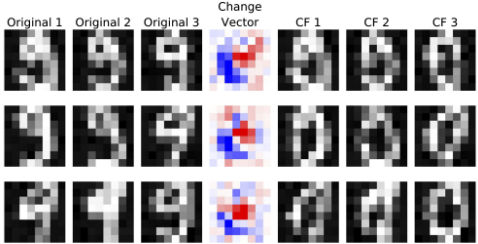
Figure 2 demonstrates our method's application to the Digits dataset, presenting group-wise counterfactual explanations for the origin class is 9, transitioning to the desired class 0. Our method clusters instances into three groups, ensuring that instances within the same group require similar modifications to achieve their counterfactuals. The first group demands substantial changes, as shown by prominent shifts in the change vector, while the third group requires fewer adjustments, indicating an easier path to the desired class. This variation underscores our method's ability to differentiate the effort required for different groups to reach the target class. This distinction demonstrates how our method tailors group-specific counterfactuals based on structural and feature differences. These findings confirm our method's capability to produce interpretable and group-specific counterfactual explanations for image data, offering insights into the transformations needed to achieve GWCFs for diverse instance groups. We provide an additional extended analysis in Appendix J.2.
5.3 Case Study: Credit Scoring with HELOC Dataset
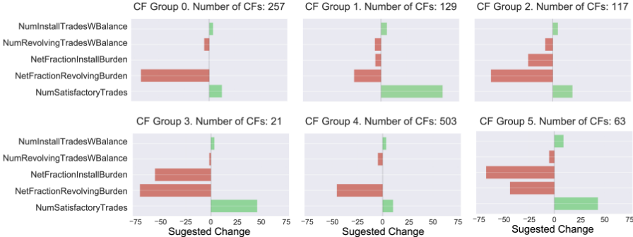
The dataset comprises HELOC credit line applications aimed at predicting whether applicants will repay their credit lines within two years. We selected five financial indicators (Number of Satisfactory Trades, Net Fraction of Revolving Burden, Net Fraction of Installment Burden, Number of Revolving Trades with Balance, Number of Installment Trades with Balance) for their potential to enable rapid behavioral adjustments. By allowing the selection of only a subset of variables, enforcing monotonicity constraints, and specifying feature ranges, our method ensures actionability by focusing on financially adjustable features within realistic limits. Detailed explanation of practical actionability implementation is provided in Appendix C. Specifically, Number of Satisfactory Trades can only increase (reflecting improved credit standing), Net Fraction of Revolving Burden and Net Fraction of Installment Burden can only decrease (indicating reduced debt utilization), Number of Revolving Trades with Balance can only decrease (showing debt consolidation), while Number of Installment Trades with Balance can change in either direction. These indicators facilitate immediate changes, such as simulating the effects of a rejected credit scenario. Our method generated CFs, optimizing them into six groups. The proposed actions are illustrated in Figure 3. The results reveal diverse group-specific recommendations. Although some groups prioritize increasing satisfactory trades, others focus on reducing revolving burdens or trades. In addition, the groups differ significantly in size, which highlights potential for subgroup analysis. A detailed interpretation is provided in Appendix J.3.
6 Conclusions
In this work, we introduced a unified method for generating counterfactual explanations at the local, group-wise, and global levels. Our approach dynamically adapts to different levels of granularity, eliminating the need for separate clustering and counterfactual generation steps. By formulating a counterfactual search as a single optimization task, we efficiently generate explanations that balance validity, proximity, and plausibility while optimizing group granularity. Additionally, we integrate probabilistic plausibility constraints within global and group-wise counterfactual explanations, ensuring that generated recourse suggestions remain realistic and actionable. The experimental results demonstrate the effectiveness of our approach across multiple datasets and classification models. In particular, we showed that our groupwise method produces a relatively small number of meaningful and interpretable groups, capturing distinct patterns within the data. Compared to state-of-the-art methods, our framework achieves superior validity while maintaining competitive plausibility and proximity. This method supports informed decision-making and advances research in model debugging and decision support systems.
Acknowledgements
Oleksii Furman, "ukasz Lenkiewicz and Maciej Zi˛eba's work was supported by the National Science Centre (Poland) Grant No. 2024/55/B/ST6/02100. Jerzy Stefanowski's work was supported by the National Science Centre (Poland) Grant No. 2023/51/B/ST6/00545.
@inproceedings{ijcai2026p65,
  title     = {Unifying Perspectives: Plausible Counterfactual Explanations on Global, Group-wise, and Local Levels},
  author    = {Furman, Oleksii and Wielopolski, Patryk and Lenkiewicz, Łukasz and Stefanowski, Jerzy and Zięba, Maciej},
  booktitle = {Proceedings of the Thirty-Fifth International Joint Conference on
               Artificial Intelligence, {IJCAI-26}},
  publisher = {International Joint Conferences on Artificial Intelligence Organization},
  editor    = {Diego Calvanese},
  pages     = {571--579},
  year      = {2026},
  month     = {8},
  note      = {Main Track},
  doi       = {10.24963/ijcai.2026/65},
  url       = {https://doi.org/10.24963/ijcai.2026/65},
}
TY - CPAPER TI - Unifying Perspectives: Plausible Counterfactual Explanations on Global, Group-wise, and Local Levels AU - Furman, Oleksii AU - Wielopolski, Patryk AU - Lenkiewicz, Łukasz AU - Stefanowski, Jerzy AU - Zięba, Maciej T2 - Proceedings of the Thirty-Fifth International Joint Conference on Artificial Intelligence, IJCAI-26 PB - International Joint Conferences on Artificial Intelligence Organization PY - 2026 SP - 571 EP - 579 DO - 10.24963/ijcai.2026/65 UR - https://doi.org/10.24963/ijcai.2026/65 ER -Copied
Machine-readable versions of this paper, for tools and AI agents:





