
RODIS: Robust Diffusion Solver to Dataset Quality in Combinatorial Optimization
Proceedings of the Thirty-Fifth International Joint Conference on Artificial Intelligence. Main Track. Pages 5263-5270.
https://doi.org/10.24963/ijcai.2026/586
© 2026 International Joint Conferences on Artificial Intelligence
Keywords
- Machine Learning: Generative models
- AI: Machine Learning
- AI: Constraint Satisfaction and Optimization
Abstract
Combinatorial optimization (CO) problems have widespread applications in science and engineering, but they present significant computational challenges. Recent advancements in generative models, particularly diffusion models, have shown promise in bypassing traditional optimization solvers by directly generating near-optimal solutions.
However, existing diffusion solvers are highly sensitive to the quality of the training dataset, particularly the number of problem instances for training and the optimality of their labels. Notably, we observe an exponential scaling law between the performance of diffusion-based solvers and the number of near-optimally labeled instances needed. When training instances are scarce or sub-optimally labeled, diffusion-based solvers suffer significant performance degradation.
To enhance the robustness of diffusion solvers to dataset quality, we propose a robust diffusion solver for combinatorial optimization capable of learning from sub-optimally labeled instances follows a two-stage generate-then-decode framework, integrating an objective-guided diffusion model, further reinforced by classifier-free guidance, to produce solutions that surpass the optimality of the training dataset.
Experiments demonstrate the improved robustness in \myalg compared to the diffusion-based solver baseline, in a range of combinatorial optimization benchmark tasks such as TSP (Traveling Salesman Problem) and MIS (Maximum Independent Set).
- [Applegate et al., 2006] David Applegate, Ribert Bixby, Vasek Chvatal, and William Cook. Concorde tsp solver, 2006.
- [Arora, 1996] Sanjeev Arora. Polynomial time approxima- tion schemes for euclidean tsp and other geometric prob- lems. In Proceedings of 37th Conference on Foundations of Computer Science, pages 2-11. IEEE, 1996.
- [Erdos et al., 1960] Paul Erdos, Alfréd Rényi, et al. On the evolution of random graphs. Publ. math. inst. hung. acad. sci, 5(1):17-60, 1960.
- [Gonzalez, 2007] Teofilo F Gonzalez. Handbook of approx- imation algorithms and metaheuristics. Chapman and Hall/CRC, 2007.
- [Graikos et al., 2022] Alexandros Graikos, Nikolay Malkin, Nebojsa Jojic, and Dimitris Samaras. Diffusion models as plug-and-play priors. Advances in Neural Information Processing Systems, 35:14715-14728, 2022.
- [Helsgaun, 2017] Keld Helsgaun. An extension of the lin-kernighan-helsgaun tsp solver for constrained travel- ing salesman and vehicle routing problems. Roskilde: Roskilde University, 12:966-980, 2017.
- [Ho and Salimans, 2022] Jonathan Ho and Tim Salimans. Classifier-free diffusion guidance. arXiv preprint arXiv:2207.12598, 2022.
- [Hoos and Stützle, 2000] Holger H Hoos and Thomas Stützle. Satlib: An online resource for research on sat. Sat, 2000:283-292, 2000.
- [Ioffe and Szegedy, 2015] Sergey Ioffe and Christian Szegedy. Batch normalization: Accelerating deep net- work training by reducing internal covariate shift. In International Conference on Machine Learning, pages 448-456, 2015.
- [Joshi et al., 2019] Chaitanya K Joshi, Thomas Laurent, and Xavier Bresson. An efficient graph convolutional net- work technique for the travelling salesman problem. arXiv preprint arXiv:1906.01227, 2019.
- [Joshi et al., 2020] Chaitanya K Joshi, Quentin Cappart, Louis-Martin Rousseau, and Thomas Laurent. Learning the travelling salesperson problem requires rethinking gen- eralization. arXiv preprint arXiv:2006.07054, 2020.
- [Kool et al., 2019] Wouter Kool, Herke Van Hoof, and Max Welling. Attention, learn to solve routing problems! In International Conference on Learning Representations, 2019.
- [Krizhevsky et al., 2010] Alex Krizhevsky, Geoff Hinton, et al. Convolutional deep belief networks on cifar-10. Un- published manuscript, 40(7):1-9, 2010.
- [Li et al., 2024] Yang Li, Jinpei Guo, Runzhong Wang, and Junchi Yan. From distribution learning in training to gradient search in testing for combinatorial optimization. Advances in Neural Information Processing Systems, 36, 2024.
- [Lin and Kernighan, 1973] Shen Lin and Brian W Kernighan. An effective heuristic algorithm for the traveling-salesman problem. Operations research, 21(2):498-516, 1973.
- [Lucas, 2014] Andrew Lucas. Ising formulations of many np problems. Frontiers in physics, 2:5, 2014.
- [Nisonoff et al., 2024] Hunter Nisonoff, Junhao Xiong, Stephan Allenspach, and Jennifer Listgarten. Unlocking guidance for discrete state-space diffusion and flow mod- els. arXiv preprint arXiv:2406.01572, 2024.
- [Olmi, 2024] Roberto Olmi. Heuristic algorithm for finding maximum independent set. https://www.mathworks.com/ matlabcentral/fileexchange/28470-heuristic-algorithm- for-finding-maximum-independent-set, 2024. MATLAB Central File Exchange. Retrieved September 11, 2024. Link
- [Qiu et al., 2022] Ruizhong Qiu, Zhiqing Sun, and Yiming Yang. Dimes: A differentiable meta solver for combinato- rial optimization problems. Advances in Neural Informa- tion Processing Systems, 35:25531-25546, 2022.
- [Sun and Yang, 2023] Zhiqing Sun and Yiming Yang. Di- fusco: Graph-based diffusion solvers for combinatorial optimization. Advances in Neural Information Processing Systems, 36:3706-3731, 2023.
- [Vaswani et al., 2017] Ashish Vaswani, Noam Shazeer, Niki Parmar, Jakob Uszkoreit, Llion Jones, Aidan N Gomez, Łukasz Kaiser, and Illia Polosukhin. Attention is all you need. In Advances in Neural Information Processing Sys- tems, volume 30, 2017.
- [Xu et al., 2019] Keyulu Xu, Weihua Hu, Jure Leskovec, and Stefanie Jegelka. How powerful are graph neural net- works? In International Conference on Learning Rep- resentations, 2019.
References were extracted automatically from the PDF and may contain errors.
Full text extracted automatically from the PDF; figures, tables and equations may differ. The PDF is the version of record.
1 Introduction
Combinatorial optimization (CO) problems require selecting optimal solutions from exponentially large search spaces and are central to many scientific and industrial applications. Classical approaches based on integer programming or handcrafted heuristics [Gonzalez, 2007; Arora, 1996] often demand substantial computation and domain expertise. Recently, generative models have emerged as a promising alternative, achieving strong performance on canonical CO problems such as the Traveling Salesman Problem (TSP) and Maximum Independent Set (MIS). In particular, diffusionbased solvers [Sun and Yang, 2023; Li et al., 2024] have achieved state-of-the-art results by leveraging supervised progressive denoising to model multi-modal solution distributions, while avoiding the sequential bottleneck of autoregressive methods and the instability of reinforcement learning.
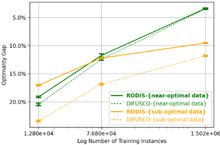
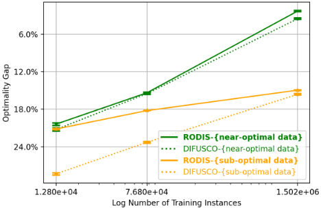
Despite their success, diffusion-based solvers are highly sensitive to training data quality. Their performance depends critically on both the number of training instances and the optimality of solution labels. As shown in Figure 2, the performance of DIFUSCO [Sun and Yang, 2023] degrades substantially when trained on limited or sub-optimally labeled data, revealing unfavorable data scaling behavior. This sensitivity poses a major challenge in practice, where collecting largescale near-optimal labels is often expensive or infeasible.
In this work, we ask whether diffusion-based solvers can be made robust to limited data and sub-optimal labels. We propose RODIS , an objective-guided diffusion framework for robust combinatorial optimization. RODIS conditions the diffusion process on the optimization objective, enabling controlled generation of solutions with higher quality than those observed during training. We further introduce a classifier-free guidance mechanism tailored to CO and adopt a generate-then-decode strategy to ensure feasibility. Experiments on TSP and MIS benchmarks demonstrate that RODIS consistently improves robustness under limited and noisy data, while retaining strong performance when highquality labels are available.
2 Problem Setup
We start with a formal problem set-up of combinatorial optimization (CO). In § 2.2, we introduce the sub-optimal training data to use in RODIS on its generation time and quality.
2.1 Combinatorial Optimization on Graphs
A lot of combinatorial optimization (CO) problems can be formulated with graphs [Lucas, 2014], so we formally formulate CO problems with graph structure by:
where x denotes the solution, f(x | G) denotes the objective function given input graph G and ci(x, G) ≤ 0 represents the set of I constraints. The goal of CO is to find the solution x satisfying (1) for any input graph G, which specifies an instance of the problem. To present our method with higher clarity, three specific CO problems are provided as examples. We start with some necessary notations for defining those problems.
| Labeller | TSP-100 | Weighted MIS-100 | ||||
|---|---|---|---|---|---|---|
| Length↓ | Gap↓ | Time ↓ | Size↑ | Gap ↓ | Time ↓ | |
| Exact Solver | 7.76 | - | 13.20 min | 135.40 | - | 40.00min (32 workers) 0.91min |
| Heuristic | 8.72 | 12.29 % | 2.10 min | 122.47 | 9.55 % | |
Notations. A graph G = ⟨V ,E⟩ consists of node features V ∈ Rn×dv , where vi ∈ Rdv is the feature of node i, and edge features E = {eij ∈ Rde | 1 ≤ i, j ≤ n}. A solution x is either a permutation or a subset of the node index set S = {1, · · · , n}; we denote its elements as x(i).
In what follows, we present rigorous formulations of two representative CO problems.
[Travelling Salesman Problem (TSP)] TSP is defined on a fully connected undirected graph G, where vi ∈ R2 is the coordinate of node i and eij = eji is the Euclidean distance between nodes i and j. The goal is to find a permutation x over all nodes minimizing the total tour length f(x | G) = ∑n-1 i=1 ex(i),x(i+1) +ex(n),x(1).
[Maximum Independent Set (MIS)] MIS seeks the largest independent set in an undirected graph G with binary edges (eij = 1 if connected). We consider both weighted (vi ∈ N∗ ) and unweighted (vi = 1) versions. The solution x ⊂ S must satisfy ex(i),x(j) = 0 for all pairs, and the objective is f(x | G) = ∑x(i)∈x vx(i).
2.2 Near-Optimal and Sub-Optimal Training Dataset
Due to the high computational complexity of CO, both solvers and heuristics are used to generate solutions. Solvers 1 can produce optimal (exact or near-optimal) solutions but are relatively expensive in computation, whereas heuristics are more computationally efficient but often yield sub-optimal solutions. In this paper, we consider the supervised dataset
1 In this paper, "solver" refers to both exact solvers or heuristic solvers that can provide exact or near-optimal solutions.
{(G, x)} under two configurations: x is the exact or nearoptimal solution of G produced by a solver or it is a suboptimal solution produced by a heuristic. Table 1 records a comparison of the labeling time and the label quality between an exact solver and a heuristic for TSP and MIS. This shows that generating a sub-optimal training dataset is significantly more inexpensive than generating a near-optimal one, at the cost of reduced label quality.
3 RODIS : Robust Diffusion Solver with Objective Guidance
Diffusion-based CO solvers [Sun and Yang, 2023; Li et al., 2024] adopt a generative perspective of solving a given problem instance G - it naturally corresponds to a conditional generation task: to generate one solution according to the distribution P(x∗ | G), which is the conditional distribution of optimal solutions given the problem instance. In this section, we start with a generalized "generate-then-decode" framework that RODIS is based on, to transform a CO problem into a generation task.
3.1 Generate-Then-Decode Framework
RODIS is primarily based on the generative perspective proposed by [Sun and Yang, 2023; Li et al., 2024], which forms a "generate-then-decode" framework: first, modeling the distribution (logits) of a binary vector using a generative model, and then decoding the final solution based on these logits. In previous work, a solution to the original CO problem can either be directly represented as a binary vector (e.g., MIS) or be closely related to one (e.g., TSP).
In this paper, we introduce a generalized "generate-thendecode" framework that has the potential to extend its applicability to a broader range of CO problems. Instead of generating a binary vector, we formulate the first stage as generating a "solution graph" G x based on the "problem graph" G. Then in the second stage a decoding algorithm h(·) is applied to solve G x so that the final solution is obtained as x = h(G x).
An intriguing observation is that the current "generatethen-decode" framework closely links to the following bilevel relaxation of the original CO:
here f and G are the same objective and problem instance in (1), and lower level problem in (2) is approximately solved by the decoding algorithm h(·) in the two-stage process. We formulate TSP and MIS under the framework as two examples. The solution graph G x = ⟨V x,Ex⟩ generated in the first stage and the solution x output in the second stage are defined as follows:
- TSP: x is a permutation of nodes in G. In G x, V x = V , i.e. the node features stayed unchanged from the problem
- graph G. In Ex, the edge between node i and j exits if and only if it is covered in the tour specified by x, i.e. ex(n),x(1) = 1 and ex(i),x(i+1) = 1 for i = 1 · · · n - 1, ei,j = 0 for the rest of positions.
- MIS: x is a subset of nodes in G. In G x,Ex = E, i.e. the edge features stayed unchanged from the problem graph G. The node feature V x have vi = 1 if node i is in the solution subset x, otherwise vi = 0.
In both TSP and MIS, x is naturally a solution to the lowerlevel problem in (2). Since the generated graph G x closely reflects the target solution, x can be recovered using simple greedy decoding [Graikos et al., 2022; Qiu et al., 2022; Sun and Yang, 2023]:
- TSP: Sort edge logits Ex by confidence and greedily add non-conflicting edges until a valid tour is formed.
- MIS: Greedily add nodes in descending order of V x logits whenever no conflict exists.
While these procedures follow prior work [Sun and Yang, 2023; Li et al., 2024], we further extend the "generate-thendecode" framework to weighted MIS by concatenating problem and solution graphs (§ 3.2). More broadly, the bi-level perspective suggests applicability to more complex CO problems by first generating a modified graph G x and then solving it with standard heuristics.
3.2 Objective-Guided DiffusionModels
In this subsection, we present RODIS method, featuring a objective-conditioned diffusion model and a guidance technique, concluded by the network architecture of RODIS .
Objective-Conditioned Diffusion Solver
To develop a diffusion model that maximally utilizes training data with sub-optimal labels, we first propose an objectiveconditioned diffusion model, which approximates P(G x | G, f(x | G)), incorporating the objective value f(x | G)) as a separate condition. The diffusion model for modeling P(G x | G, f(x | G)) follows the discrete diffusion formulation in [Sun and Yang, 2023] for its forward process. W.L.O.G, we only present the process for generating edges in G x, generating nodes is similar.
Categorical noise is progressively added to Ex sampled from P(Ex | G) by formula (3), generating a sequence of latents Ex 0:T := Ex 0 ,Ex 1 , · · · ,Ex T such that Ex 0 := Ex and
where Cat(·, p) denotes categorical distribution, Qt's are transition kernel for categorical variables. The sampling process is equivalent to
The backward denoising process of our model is objective conditioned, which denoises Ex t to generate the preceding variable Ex t-1 , based on 4 inputs: the current state Ex t , the problem instance G, the objective f(x | G) and the time step t. The denoiser is learned by model ϕθ, aiming to align its prediction to the input solution Ex 0 , thus the loss for training ϕθ is:
The architecture of objective-guided denoiser ϕθ will be introduced in §3.2. During inference, we first set a target objective ftar and start the backward diffusion process by sampling ET from the uniform distribution. Then iteratively at each time step t, denoting the prediction of ϕθ(Et, G, ftar, t) as ˆE0, the one-step predecessor Et-1 can be generated from the following posterior distribution:
where ⊙ denotes the element-wise multiplication. After T iterations, the recovered solution graph G0 is expected to have the same distribution as P(G x | G, ftar) so that the solution decoded out from G0 has objective equal to ftar, if the diffusion model approximates the ground truth distribution well. A theoretical choice of ftar is the optimal objective for the original problem, f ∗ = minx f(x | G). In practice, one can take ftar as a model hyper-parameter and grid search for proper ftar with a validation set (§ 4.2).
Reinforcing with Guidance
The performance of objective conditioning can be further reinforced by the guidance mechanism [Ho and Salimans, 2022; Nisonoff et al., 2024]. In the sequel, we propose a classifier-free guidance for categorical diffusion model with discrete state, compatible with our objective-conditioned diffusion model (Algorithm 1).
Ideally, we want to generate from P(G x | G, f ∗ ) with f ∗ being the optimal objective for problem G. Diffusion model approximates this distribution by iteratively sampling from P (G x t-1 | G x t , G, f ∗ ) for discrete time steps t ∈ [T], to achieve this, P(G x | G x t , G, f ∗ ) is the key quantity to learn by diffusion model as demonstrated in (5). P(G x | G x t , G, f ∗ ) contains the information about objective value and Bayesian rule suggests:
where P(G x t-1 | G x t , G) on the RHS is the unconditioned probability to denoise G x t . (6) shows the difference between conditioned and unconditioned denoising probability
Algorithm 1 Training
- 1: Input: Training dataset: D = {(G, x, f(x))}
- 2: Initialize: denoising network ϕθ(·),
- mask probability p, T ← total diffusion steps,
{Qt}, {Qt } ← noise transitions.
- 3: Pre-process the Training Data: represent x as solution graph Gx = ⟨V x , Ex ⟩ as in § 3.1, and obtain D = {(G, G x , f(x))}.
- 4: for each training step do
- 5: Sample t from [0, T].
- 6: Sample s ∼ Ber(p).
- 7: Add Noise:
- 8: Update θ with one gradient step w.r.t loss (8).
- 9: end for
is P(f ∗ | G x t , G). Thus, P(f ∗ | G x t , G) suggests the the direction to improve the optimality of generated solutions and quantitatively it equals to P(Gx t-1 |Gx t ,G,f ∗ ) P (Gx t-1 |Gx t ,G) , which can be easily seen by dividing the denominator from (6) on both sides. Therefore, we propose to further enhance the guidance of objective by denoising with the following probability at each step:
In (7), Z is a normalizing factor and γ ≥ 0 controls the strength of guidance.
To facilitate classifier-free guidance as (7), we jointly train an unconditioned denoiser to approximate P(G x t-1 | G x t , G) together with the original conditioned one. Therefore, for training an objective-directed diffusion model with classifierfree guidance, we modify the previous loss in (4) to be
in which the expectation is taken over t ∼ Unif ((0, T ]) and s ∼ Bernoulii (p). Here s is a random seed for determining which samples are held out for training unconditioned denoiser, and an empirical choice of p is 0.1. It is worth mentioning that both conditioned and unconditioned training share the same model ϕθ: if a sample is sent to unconditioned training, then it will go through the forward pass of ϕθ with the objective condition being masked.
The pseudo-code of training and inference from the objective-guided diffusion model is provided in Algorithm 1 and Algorithm 2.
Computation in Inference. When γ = 0, the objectiveconditioned diffusion model in RODIS runs without guidance, requiring one forward pass of the denoising network per
Algorithm 2 Inference
- 1: Input: denoising network ϕθ(·), problem G = ⟨V ,E⟩, target objective ftar, guidance strength γ, decoding algorithm h(·).
- 2: Initialize: T ← total diffusion steps
- N ← # of nodes in G,
- {Qt}, {Qt } ← noise transitions,
- 3: Sample: ET ← {ei,j}N×N, ei,j ∼ Ber( 12 ).
- 4: for t = T, T -1, · · · , 1 do
- 6: t ← t - 1.
- 7: end for
- 8: Decode: x← h(G x ), Gx = ⟨V ,E0⟩.
step. When the guidance mechanism is activated with γ ≥ 0, inference requires two forward passes of the denoising network.
Objective-Guided Denoising Network
In (8), our objective-directed denoiser ϕθ(G x t , G, f(x), t) takes as input the noisy solution graph G x t , the problem graph G, the objective value of solution f(x), the time step t, to predict the clean solution graph G x 0 . Since the denoiser should support predict both node and edge features in the solution graph, we adopt an anisotropic graph neural network [Joshi et al., 2019; Qiu et al., 2022; Sun and Yang, 2023] as the backbone, which can produce embeddings for both nodes and edges. To incorporate and process the objective information, we propose the following architecture for objective-directed graph denoiser, which is also illustrated in Fig.4.
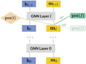
Objective-AwareGraph-BasedDenoiser. Let hℓi andmℓij denote the node and edge features at layer ℓ for node i and edge ij. To process timestep t and objective f(x), we adopt the positional encoding [Vaswani et al., 2017] and denote: t = pos(t) and f = pos(f(x)). The features at the next layer is propagated with an anisotropic message passing scheme, engaging the positional encodings of both timestep t and objective f(x):
| Method | Data Label | TSP-50 (12800) | TSP-50 (76800) | TSP-50 (1502000) | |||
|---|---|---|---|---|---|---|---|
| Length↓ | Gap↓ | Length↓ | Gap ↓ | Length↓ | Gap ↓ | ||
| Concorde | - | 5.60 | - | 5.60 | - | 5.60 | - |
| DIFUSCO | Solver | 6.74 | 20.36 % | 6.29 | 12.32 % | 5.79 | 3.39 % |
| RODIS (γ = 0) | Solver | 6.67 | 19.10 % | 6.25 | 11.60 % | 5.79 | 3.39 % |
| DIFUSCO | Heuristic | 6.91 | 23.39 % | 6.54 | 16.79 % | 6.26 | 11.79 % |
| RODIS (γ = 0) | Heuristic | 6.78 | 21.07 % | 6.38 | 13.93 % | 6.15 | 9.82 % |
| RODIS | Heuristic | 6.55 | 16.96% | 6.28 | 12.14% | 6.11 | 9.11% |
| Method | Data Label | TSP-100 (12800) | TSP-100 (76800) | TSP-100 (1502000) | |||
|---|---|---|---|---|---|---|---|
| Length↓ | Gap↓ | Length↓ | Gap ↓ | Length↓ | Gap ↓ | ||
| Concorde | - | 7.68 | - | 7.68 | - | 7.68 | - |
| DIFUSCO | Solver | 9.32 | 21.35 % | 8.87 | 15.49 % | 7.95 | 3.52 % |
| RODIS (γ = 0) | Solver | 9.25 | 20.18% | 8.86 | 15.36 % | 7.85 | 2.21% |
| DIFUSCO | Heuristic | 9.86 | 28.39 % | 9.47 | 23.31 % | 8.88 | 15.63 % |
| RODIS (γ = 0) | Heuristic | 9.69 | 26.17 % | 9.32 | 21.35 % | 8.86 | 15.36 % |
| RODIS | Heuristic | 9.30 | 21.09% | 9.08 | 18.23% | 8.83 | 14.97 % |
where in layer ℓ, U ℓ , V ℓ , P ℓ , Qℓ , Rℓ ∈ Rd×d and MLP(·) are learnable. MLP(·) with subscripts m, t, f all denote a 2-layer multi-layer perceptron. α, BN, A, σ denote the ReLU [Krizhevsky et al., 2010] activation, batch normalization [Ioffe and Szegedy, 2015], aggregation function SUM pooling [Xu et al., 2019] and sigmoid function, respectively. ⊙ is the Hadamard product, Ni denotes the neighborhoods of node i. We use 12 layers with hidden dimension d = 256 following [Sun and Yang, 2023]. Lastly, a Sigmoid activation is applied to the final layer embeddings of nodes or edges, which is then to predict a binary cross entropy loss between candidate solution graph vs. input solution graph.
Double Graph Conditioning. It is worth noticing that our denoiser ϕθ(G x t , G, f(x), t) takes two graphs as input: the problem graph G and the noisy solution graph G x t . To pass both graphs into the anisotropic GNN above, we concatenate the positional encoding of node/edge features in both graphs: suppose G = ⟨V ,E⟩ and G x t = ⟨V x t ,Ex t ⟩, we pass h0i = (pos(V(i)), pos(V x t,(i) )) and m0ij = (pos(E(i,j)), pos(Ex t,(i,j) )) into the GNN layers.
4 Experiments
4.1 Experimental Setup
In this section, we provide experiments to study the robustness of RODIS . We evaluate the performance RODIS on two benchmarks: TSP and (weighted and unweighted) MIS, when faced with limited number of training instances and sub-optimal label quality. The setup for data collection including the choice of heuristics, metrics and baselines are specified in separate subsections for each problem. Hyperparameters are as follows.
Hyper-parameters in diffusion models. Following DIFUSCO [Sun and Yang, 2023], the models for all problems are trained with 1000 denoising steps, i.e., T = 1000, while during inference, we adopt 50 inference steps. We provide in § 4.2 an ablation study on the choices of other two important hyper-parameters for inference: the guidance strength and the target objective value.
4.2 Ablation Study: the Effect of Guidance
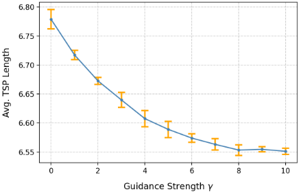
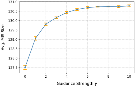
Guidance Strength. We investigate the effectiveness of guidance strength γ in (7). To efficiently evaluate this choice, we utilize the TSP-50 and Weighted MIS-100 benchmarks and train both models with 12800 instances. We evaluate the model performance on test set, varying the guidance strength by setting γ ∈ {0, 1, 2, · · · , 10} and taking denoising step with guidance as (7) specifies; evaluation results across 5 random seeds are plotted in Fig.6. When γ = 0, the model degrades to the basic objective-conditioned diffusion model (Alg. 1), it can be seen from Fig.6 that enlarging guidance γ improves the baseline performance reported at γ = 0. It demonstrates that guidance effectively enhances the model performance, guiding the denoising process towards highobjective value region in the solution space.
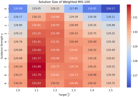
Target Objective Value. We also evaluate the impact of target objective value ftar at inference time. Fig. 7 is a heatmap on the average objective of generated solutions when jointly varying target ftar and strength γ. Recall from § 3.2, a theoretical choice of ftar is the optimal objective value f ∗ . While empirically, we observe that good choices of ftar live in a wild range above f ∗ (for maximization) or below f ∗ (for minimization), see Fig. 7. Here we provide an reference practice for choosing ftar: replace f ∗ with the average optimal objective value in a small validation set and search the multiplication factor from [1.1, · · · , 1.5] for maximization or [0.5, 0.6, · · · , 0.9] for minimization and fix the ftar for inference. The best choice of ftar and γ is model specific, one can jointly search the two and freely decide how many values to search. ftar and γ will be fixed during inference. All experiment results for RODIS with guidance enabled is reported under fixed ftar and γ for all testing instances.
4.3 Experiments on TSP
Datasets. Following [Kool et al., 2019; Joshi et al., 2019], TSP instances are generated by uniformly sampling n nodes from [0, 1]2 . Training instances are labeled by heuristic Farthest Insertion and solver Concorde[Applegate et al., 2006] (TSP-50/100) or LKH-3[Helsgaun, 2017] (TSP500/1000). We train with three dataset sizes: 12800, 76800, and 1502000 instances for TSP-50/100, and the same for TSP-500/1000. Test sets contain 1280 instances for TSP50/100 [Kool et al., 2019; Joshi et al., 2020] and 128 for TSP-500/1000.
Metrics. We report (i) Length: the average tour length; and (ii) Gap: the average suboptimality gap w.r.t. Concorde (TSP-50/100) or LKH-3 (TSP-500/1000).
Baselines. We compare RODIS to DIFUSCO under both near-optimal and sub-optimal labels, using the same greedy decoding without 2-opt [Lin and Kernighan, 1973] refinement.
Results and Analysis. Results are in Tables 2, 3, and 5. RODIS outperforms DIFUSCO across all sizes when trained with heuristic labels. Notably, on TSP-50 with 12800 and 76800 instances, RODIS with heuristic labels even surpasses DIFUSCO with solver labels. The scaling curves in Figure 2[Right] and Figure 5 show that RODIS retains strong performance under solver-labeled data (solid vs. dotted green) while significantly mitigating degradation under suboptimal data (solid vs. dotted orange), even outperforming DIFUSCO with near-optimal data in the data-scarce regime (12800 ∼ 76800). Similar trends hold for TSP-100 and TSP500/1000.
| Method | Data Label | WeightedMIS-100 | SATLIB | ER[700-800] | ||||||
|---|---|---|---|---|---|---|---|---|---|---|
| Size↑ | Gap↓ | Size↑ | Gap↓ | Size↑ | Gap↓ | |||||
| Kamis | - | - | - | - | - | 44.73 | - | |||
| Gurobi | - | 135.40 | - | 425.45 | - | - | - | |||
| findMIS | - | 122.37 | 9.62 % | 421.50 | 0.93 % | 39.47 | 11.76 % | |||
| DIFUSCO | Solver | 133.60 | 1.33 % | 423.09 | 0.55% | 40.93 | 8.51 % | |||
| RODIS | Solver | 133.79 | 1.19% | (-0.12%) | 421.74 | 0.87% | (+0.32%) | 41.41 | 7.40% | (-1.11%) |
| DIFUSCO | Heuristic | 121.78 | 10.06 % | 420.46 | 1.17 % | 40.77 | 8.85 % | |||
| RODIS | Heuristic | 130.66 | 3.63% | (-6.43%) | 420.91 | 1.07% | (-0.10%) | 41.13 | 8.04% | (-0.81%) |
| Method | Data Label | TSP-500 | TSP-1000 | ||
|---|---|---|---|---|---|
| Length↓ | Gap↓ | Length↓ | Gap ↓ | ||
| LKH-3 | - | 16.54 | - | 23.18 | - |
| DIFUSCO | Solver | 18.47 | 11.67 % | 27.44 | 18.38 % |
| RODIS (γ = 0) | Solver | 18.31 | 10.70 % | 27.60 | 19.07% |
| DIFUSCO | Heuristic | 21.60 | 30.59 % | 32.46 | 40.03 % |
| RODIS | Heuristic | 20.73 | 25.33% | 31.82 | 37.27% |
4.4 Experiments onMIS
Datasets. We evaluate on three MIS datasets: Weighted MIS-100, SATLIB [Hoos and St ¨utzle, 2000], and unweighted ER graphs [Erdos et al., 1960] with 700 ∼ 800 nodes. Since [Sun and Yang, 2023] only addressed unweighted MIS, we introduce a weighted MIS-100 dataset of ER graphs (100 nodes, connection probability 0.15, weights ∼ (5, 2) rounded to integers), with 12800/128/1280 train/validation/test splits. SATLIB 2 and ER[700-800] follow the same data and test setup as [Qiu et al., 2022; Sun and Yang, 2023; Li et al., 2024]. Training labels are generated by the polynomial heuristic findMIS [Olmi, 2024].
Metrics. We report (i) Size: the average (weighted) independent set size; and (ii) Gap: the suboptimality gap w.r.t. Gurobi 3 or Kamis 4 .
Results and Analysis. Results are in Table 4. Under near-optimal labels, RODIS matches or slightly outperforms DIFUSCO across all datasets. Under sub-optimal labels, RODIS significantly mitigates the performance drop on Weighted MIS-100. The improvement on SATLIB is marginal, as all methods already achieve near-zero gaps. Notably, RODIS outperforms findMIS-its own labeling heuristic-by 6% on Weighted MIS-100 and 3% on ER[700800], demonstrating extrapolation beyond training label quality. On ER[700-800], RODIS with heuristic labels even surpasses DIFUSCO with solver labels.
5 Conclusions
We identified a data scaling law in training diffusion solvers for CO, showing high sensitivity to data quantity and label quality. To improve robustness, we proposed RODIS , a generate-then-decode framework with an objective-guided diffusion model reinforced by classifier-free guidance. Experiments show that RODIS matches DIFUSCO on highquality data and significantly outperforms it under data-scarce or sub-optimally labeled settings.
@inproceedings{ijcai2026p586,
  title     = {RODIS: Robust Diffusion Solver to Dataset Quality in Combinatorial Optimization},
  author    = {Yuan, Hui and Hua, Zhigang and Li, Zihao and Xu, Qi and Cong, Weilin and Xie, Yan and Li, Taihui and Jin, Rong and Yang, Shuang and Long, Bo},
  booktitle = {Proceedings of the Thirty-Fifth International Joint Conference on
               Artificial Intelligence, {IJCAI-26}},
  publisher = {International Joint Conferences on Artificial Intelligence Organization},
  editor    = {Diego Calvanese},
  pages     = {5263--5270},
  year      = {2026},
  month     = {8},
  note      = {Main Track},
  doi       = {10.24963/ijcai.2026/586},
  url       = {https://doi.org/10.24963/ijcai.2026/586},
}
TY - CPAPER TI - RODIS: Robust Diffusion Solver to Dataset Quality in Combinatorial Optimization AU - Yuan, Hui AU - Hua, Zhigang AU - Li, Zihao AU - Xu, Qi AU - Cong, Weilin AU - Xie, Yan AU - Li, Taihui AU - Jin, Rong AU - Yang, Shuang AU - Long, Bo T2 - Proceedings of the Thirty-Fifth International Joint Conference on Artificial Intelligence, IJCAI-26 PB - International Joint Conferences on Artificial Intelligence Organization PY - 2026 SP - 5263 EP - 5270 DO - 10.24963/ijcai.2026/586 UR - https://doi.org/10.24963/ijcai.2026/586 ER -Copied
Machine-readable versions of this paper, for tools and AI agents:





