
A Fast and Unified Partial Dependence Plot Algorithm
Proceedings of the Thirty-Fifth International Joint Conference on Artificial Intelligence. Main Track. Pages 5048-5056.
https://doi.org/10.24963/ijcai.2026/562
Keywords
- Machine Learning: Explainable/Interpretable machine learning
- Machine Learning: Game Theory
- Machine Learning: Ensemble methods
Abstract
Partial Dependence Plots (PDPs) visualize how changes in a single feature affect the average model prediction. They are widely used in practice to interpret decision tree ensembles and other machine learning models. Joint-PDPs extend this idea to pairs of features, revealing their combined effect. Partial Dependence Interaction Values (PDIVs) measure feature interactions. The Any-Order-PDIVs task computes these interactions for every feature subset across all rows of the dataset.
We introduce WOODELF++, a unified and efficient approach for computing all these useful explainability tools on decision tree ensembles, building on WOODELF, an algorithm for efficient SHAP computation. By deriving suitable metrics over pseudo-Boolean functions, WOODELF++ can compute PDPs (exact and approximate), Joint-PDPs, and Any-Order-PDIVs in a unified framework. Our method delivers substantial complexity improvements over the state of the art, including an exponential gain for Any-Order-PDIVs. Additionally, we introduce and efficiently compute Full PDPs, which leverage the model’s split thresholds to faithfully capture its behavior across all possible feature values.
WOODELF++ is implemented in pure Python and supports GPU acceleration. On a dataset with 400,000 rows, WOODELF++ computes PDP and Joint-PDP up to 6x faster than the state of the art and up to five orders of magnitude faster than scikit-learn. For Any-Order-PDIVs, the gap is even larger: WOODELF++ computes all interaction values in 5 minutes, while the state of the art is estimated to require over 1,000,000 years.
- [Apley and Zhu, 2020] Daniel W Apley and Jingyu Zhu. Vi- sualizing the effects of predictor variables in black box su- pervised learning models. Journal of the Royal Statisti- cal Society Series B: Statistical Methodology, 82(4):1059- 1086, 2020.
- [Blockeel et al., 2023] Hendrik Blockeel, Laurens Devos, Benoît Frénay, Géraldin Nanfack, and Siegfried Nijssen. Decision trees: from efficient prediction to responsible ai. Frontiers in Artificial Intelligence, Volume 6 -2023, 2023.
- [Caruana et al., 2015] Rich Caruana, Yin Lou, Johannes Gehrke, Paul Koch, Marc Sturm, and Noemie Elhadad. Intelligible models for healthcare: Predicting pneumonia risk and hospital 30-day readmission. In Proceedings of the 21th ACM SIGKDD International Conference on Knowledge Discovery and Data Mining, KDD '15, page 1721-1730, New York, NY, USA, 2015. Association for Computing Machinery.
- [Cook et al., 2021] Thomas Cook, Greg Gupton, Zach Modig, and Nathan Palmer. Explaining machine learning by bootstrapping partial dependence functions and shapley values. The Federal Reserve Bank of Kansas City Research Working Papers, 11 2021.
- [Cutler et al., 2007] D. Richard Cutler, Thomas C. Ed- wards Jr., Karen H. Beard, Adele Cutler, Kyle T. Hess, Jacob Gibson, and Joshua J. Lawler. Random forests for classification in ecology. Ecology, 88(11):2783-2792, 2007.
- [Friedman, 2001] Jerome H. Friedman. Greedy function ap- proximation: A gradient boosting machine. The Annals of Statistics, 29(5):1189 -1232, 2001.
- [Gnat, 2024] Sebastian Gnat. Determining the influence of real estate features on prices with partial dependence plots: A case study in szczecin, poland. Real Estate Management and Valuation, 32(4):105-116, 2024.
- [Goldstein et al., 2015] Alex Goldstein, Adam Kapelner, Justin Bleich, and Emil Pitkin. Peeking inside the black box: Visualizing statistical learning with plots of individ- ual conditional expectation. journal of Computational and Graphical Statistics, 24(1):44-65, 2015.
- [Hiabu et al., 2022] Munir Hiabu, Josephine T. Meyer, and Marvin N. Wright. Unifying local and global model expla- nations by functional decomposition of low dimensional structures. ArXiv, abs/2208.06151, 2022.
- [Jibiki and Fukuda, 2024] Taichi Jibiki and Shinji Fukuda. Temporal variables improve a spatiotemporal species dis- tribution model for the non-native freshwater fish candidia temminckii. iScience, 27(4), Apr 2024.
- [kag, 2019] Ieee-cis fraud detection dataset, 2019. https:// www.kaggle.com/c/ieee-fraud-detection. [kdd, 1999] Kdd cup 1999 data, 1999. https://kdd.ics.uci. edu/databases/kddcup99/kddcup99.html. Link
- [Ke et al., 2017] Guolin Ke, Qi Meng, Thomas Finley, Taifeng Wang, Wei Chen, Weidong Ma, Qiwei Ye, and Tie-Yan Liu. Lightgbm: A highly efficient gradient boost- ing decision tree. In I. Guyon, U. Von Luxburg, S. Bengio, H. Wallach, R. Fergus, S. Vishwanathan, and R. Garnett, editors, Advances in Neural Information Processing Sys- tems, volume 30.
- Curran Associates, Inc., 2017.
- [Liu et al., 2025] Jinyang Liu, Tessa Steensgaard, Marvin N. Wright, Niklas Pfister, and Munir Hiabu. Fast estimation of partial dependence functions using trees. In Aarti Singh, Maryam Fazel, Daniel Hsu, Simon Lacoste-Julien, Fe- lix Berkenkamp, Tegan Maharaj, Kiri Wagstaff, and Jerry Zhu, editors, Proceedings of the 42nd International Con- ference on Machine Learning, volume 267 of Proceed- ings of Machine Learning Research, pages 39496-39534. PMLR, 13-19 Jul 2025.
- [Muschalik et al., 2023] Maximilian Muschalik, Fabian Fu- magalli, Rohit Jagtani, Barbara Hammer, and Eyke Hüllermeier. ipdp: On partial dependence plots in dy- namic modeling scenarios. In Luca Longo, editor, Ex- plainable Artificial Intelligence, pages 177-194, Cham, 2023. Springer Nature Switzerland.
- [Nadel and Wettenstein, 2026a] Alexander Nadel and Ron Wettenstein. From decision trees to boolean logic: A fast and unified shap algorithm. Proceedings of the AAAI Con- ference on Artificial Intelligence, 40(29):24476-24485, Mar. 2026.
- [Nadel and Wettenstein, 2026b] Alexander Nadel and Ron Wettenstein. From decision trees to boolean logic: A fast and unified shap algorithm (extended arxiv version), 2026.
- [Nadel, 2020] Alexander Nadel. On optimizing a generic function in sat. In 2020 Formal Methods in Computer Aided Design (FMCAD), pages 205-213, 2020.
- [Parr and Wilson, 2020] Terence Parr and James D. Wilson. Technical report: Partial dependence through stratifica- tion, 2020.
- [Pedregosa et al., 2011] F. Pedregosa, G. Varoquaux, A. Gramfort, V. Michel, B. Thirion, O. Grisel, M. Blon- del, P. Prettenhofer, R. Weiss, V. Dubourg, J. Vanderplas, A. Passos, D. Cournapeau, M. Brucher, M. Perrot, and E. Duchesnay. Scikit-learn: Machine learning in Python. Journal of Machine Learning Research, 12:2825-2830, 2011.
- [Ribeiro et al., 2016] Marco Tulio Ribeiro, Sameer Singh, and Carlos Guestrin. "Why Should I Trust You?": Ex- plaining the predictions of any classifier. In Proceedings of the 22nd ACM SIGKDD International Conference on Knowledge Discovery and Data Mining, KDD 16, pages 1135-1144, New York, NY, USA, 2016. Association for Computing Machinery.
- [Shapley, 1953] L. S. Shapley. A value of n-person games. Contributions to the Theory of Games, page 307-317, 1953.
- [Sudjianto et al., 2023] Agus Sudjianto, Aijun Zhang, Zebin Yang, Yu Su, and Ningzhou Zeng. Piml toolbox for in- terpretable machine learning model development and di- agnostics. arXiv, 2023.
- [Yasodhara et al., 2021] Angeline Yasodhara, Azin Asgar- ian, Diego Huang, and Parinaz Sobhani. On the trustwor- thiness of tree ensemble explainability methods. In Ma- chine Learning and Knowledge Extraction: 5th IFIP TC 5, TC 12, WG 8.4, WG 8.9, WG 12.9 International Cross- Domain Conference, CD-MAKE 2021, Virtual Event, Au- gust 17-20, 2021, Proceedings, Berlin, Heidelberg, 2021. Springer-Verlag.
- [Zern et al., 2023] Artjom Zern, Klaus Broelemann, and Gjergji Kasneci. Interventional shap values and interac- tion values for piecewise linear regression trees. Pro- ceedings of the AAAI Conference on Artificial Intelligence, 37(9):11164-11173, Jun. 2023.
- [Zhang and Jang, 2005] Byoung-Tak Zhang and Ha-Young Jang. Molecular learning of wdnf formulae. In Alessan- dra Carbone and Niles A. Pierce, editors, DNA Computing, 11th International Workshop on DNA Computing, DNA11, Revised Selected Papers, volume 3892 of Lecture Notes in Computer Science, pages 427-437. Springer, 2005.
References were extracted automatically from the PDF and may contain errors.
Full text extracted automatically from the PDF; figures, tables and equations may differ. The PDF is the version of record.
1 Introduction
As decision tree ensembles are widely used in real-world applications [Blockeel et al., 2023], understanding their predic-
1 WOODELF++ was migrated to the WOODELF GitHub package:
https://github.com/ron-wettenstein/woodelf
Extended version of this work: https://arxiv.org/abs/2605.14578
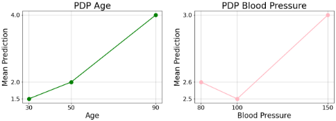
Figure 1: PDP examples.
Figure 2: Naive computation of the PDVs required to plot the PDPs in Fig. 1, carried out according to Def. 1.
tions is crucial for trust and decision-making [Yasodhara et al., 2021; Ribeiro et al., 2016]. This paper accelerates the computation of three widely used attribution metrics for decision tree ensembles: Partial Dependence Plot, Joint Partial Dependence Plot, and Partial Dependence Interaction Value.
1.1 Partial Dependence Plot (PDP)
A PDP [Friedman, 2001] illustrates how a model's average prediction varies with changes in a specific feature. For example, Fig. 1a shows that the average prediction increases with age. PDPs are widely used in many scientific domains such as healthcare [Caruana et al., 2015], ecology [Cutler et al., 2007; Jibiki and Fukuda, 2024], and economics [Gnat, 2024].
A PDP is a line plot of several PDVs (Def. 1).
Definition 1 (Partial Dependence Value (PDV)). A PDV measures the average prediction of a model M when a feature fj is fixed to a given value v. For a dataset B:
k: #selected values to plot; f: #features; F: Max number of features in a single tree; n: #samples (rows); T: #trees; D: tree depth; L: leaves per tree.
Figure 3: Notations.
To construct a PDP for feature fj , we select k possible values of fj, compute their PDVs, and plot them. The selected values are typically sampled from B[fj] or evenly spaced across its range.
For each feature fa and samples {a1, . . . ak}:
The naive way to construct these plots is to compute each PDV separately using Formula 1 (see Fig. 2). The overall complexity of computing PDPs for all features using this method is O(kfnTD) (see Fig. 3 for notation). This naive approach remains the standard in widely used frameworks such as scikit-learn [Pedregosa et al., 2011] and PiML [Sudjianto et al., 2023].
[Friedman, 2001] also introduced a faster approach that
approximates the PDVs, which we discuss in detail in Sec. 3. Several extensions of PDPs have been proposed. Individual Conditional Expectation (ICE) [Goldstein et al., 2015] plots can be viewed as PDPs computed for a single data row, revealing variation in feature effects across samples. Accumulated Local Effects (ALE) [Apley and Zhu, 2020] modifies the PDV computation by focusing on rows with feature values similar to v. A comparative analysis of PDPs, ALE, and Shapley values is presented in [Cook et al., 2021]. Additionally, iPDP [Muschalik et al., 2023] handles dynamic models that evolve over time, and StratPD [Parr and Wilson, 2020] takes a different approach: instead of interpreting the model, it generates plots that directly explain the training data.
1.2 Joint Partial Dependence Plot (Joint-PDP)
The concept of Partial Dependence Values extends naturally to feature sets: instead of fixing a single feature, we fix a set of features to chosen values - see Def. 2.
Definition 2 (Partial Dependence Value (PDV) on sets). PDV on a subset of features F = {f1, . . . , fh}, set of values V = {v1, . . . , vh} (write V [fi] = vi for the value of fi) and a dataset B is defined as follows:
To visualize the joint contribution of a feature pair, it is useful to plot their PDVs. For features fa, fb with sampled values {a1, . . . , ah} and {b1, . . . , bh}, Joint-PDP computes:
The naive approach, also used by scikit-learn, computes the PDV for every feature pair and value by fixing the pair to specific values and evaluating the model prediction (similar to Fig. 2, but fixing two features instead of one). This results in a time complexity of O(k2 f 2nTD).
1.3 Partial Dependence Interaction Value (PDIV)
It is often useful to decompose the joint effect of features into their individual effects and the effect of their interactions. PDIVs (Def. 3) do exactly this.
Definition 3 (Partial Dependence Interaction Value (PDIV)). A PDIV quantifies the interaction effect among the features F = {f1, . . . , fh} when their values are fixed to V = {v1, . . . , vh} (with V [fi] = vi). PDIVs on dataset B are defined as follows:
For example: PDIV{4,1,6},{f2,f5,f8} = PDV{4,1,6},{f2,f5,f8} -PDV{4,1},{f2,f5} - PDV{1,6},{f5,f8} - PDV{4,6},{f2,f8} +PDV{4},{f2} + PDV{1},{f5} + PDV{6},{f8} - PDV{},{}
Summing all interaction values over subsets of F reconstructs the PDV of F . Moreover, [Hiabu et al., 2022] showed that the Shapley value of a feature fi is a weighted sum of the PDIVs of all subsets S such that fi ∈ S.
The Any-Order-PDIVs task computes PDIVs for each row c in the explained data C, across all feature subsets. Let c|S = {c[fi] : fi ∈ S}, then the Any-Order-PDIVs task computes:
An acceptable result for the Any-Order-PDIVs task is to return all non-zero PDIVs. A naive method runs predictions on the background data B (see Def 3, for simplicity, we assume |B| = |C| = n), for every feature subset S ⊆ F (2f subsets in total), and for every explained sample c ∈ C. This results in a total complexity of O(2f n2TD).
1.4 FastPD
FastPD [Liu et al., 2025] is the current state-of-the-art tool for computing Any-Order-PDIVs. It exploits the structure and additivity of decision-tree ensembles to improve performance, achieving two main complexity improvements.
- By processing each tree independently, FastPD reduces 2f to 2F . This is beneficial, as the number of features used in a tree (F ) is typically much smaller than the total number of features (f).
- FastPD preprocessing reduces the data-size term from O(mn) to O(m + n), where m = |B| and n = |C|.
Overall, the complexity of FastPD for computing Any-OrderPDIVs is O (T 2D+F (n + m)). FastPD can also compute interaction values up to order s in complexity:
This complexity was not discussed in [Liu et al., 2025]; we derived it ourselves and verified it empirically. Further details are provided in the supplementary material.
The GLEX package 2 implements the FastPD algorithm in R. Although FastPD theoretically supports separate background (B) and consumer (C) datasets, this option is not available in GLEX. For our experiments, we extended the package to support this setting while preserving its efficient implementation strategy. FastPD can also compute PDP in O(T2D F(n + k)) and Joint-PDP in O(T2D F 2 (n + k2 )). This is done by computing first-order interactions for PDP and up to second-order interactions for Joint-PDP, and then reconstructing the PDVs from these interactions.
2 GLEX GitHub: https://github.com/PlantedML/glex
| Task | scikit-learn | FastPD | WOODELF++ |
|---|---|---|---|
| PDP, Sect. 3 Any-Order-PDIVs, Sect. 5 | O(kf nT D) | O(T 2D F (n + k)) O(2FnT ) | O(nT L + kT LD + T L2DD) O(n2D T L + 4D T L) |
| - | |||
| Joint-PDP, Sect. 6 | O(k2 f 2nTD) | O(T2D F 2 (n+k2 log(f))) | O(k2 f 2 log(f)+nTL+k2 log(f)TLD2 +TL2DD2 ) |
1.5 Contributions
Building on our previous work, WOODELF [Nadel and Wettenstein, 2026a], we formulate PDP, Joint-PDP, and AnyOrder-PDIVs as cooperative-game metrics and introduce WOODELF++ for their efficient computation on decision tree ensembles. Our contributions include:
- PDP and Joint-PDP speedup: We construct consumer datasets that enable efficient computation of PDP and Joint-PDP using local-attribution methods. We apply this approach to both WOODELF++ and FastPD, enhancing both methods. On large datasets, WOODELF++ is about 6× faster than FastPD.
- Exponential complexity improvement for AnyOrder-PDIVs: In the worst case, where all splits use distinct features (F = 2D ), FastPD Any-Order-PDIVs complexity has a 22D dependence, while WOODELF++ depends only on 4D . We demonstrate this gap empirically: WOODELF++ completes Any-Order-PDIVs on 400000 samples in just 5 minutes, whereas FastPD is estimated to take 1000000 years for this task.
- Full PDP:We introduce a novel method for selecting the k plotted values in a PDP, yielding full PDP - a plot that displays the PDV for any possible feature value. Our speedups make it feasible to compute these plots for all model features within practical runtimes.
- PDP Approximation: We demonstrate how WOODELF++ can be used to compute approximate PDPs, establishing a simple connection between approximate PDPs, exact PDPs, and Path-Dependence SHAP.
2 Preliminaries
2.1 Pseudo Boolean Functions
We remind the reader of Pseudo Boolean (PB) functions [Nadel, 2020] and their representation in Weighted Disjunctive Normal Form (WDNF) [Zhang and Jang, 2005], followed by the linearity property in this context.
Definition 4 (PB Function). A Pseudo Boolean (PB) function is a function of the form F(x1, . . . , xh) : {0, 1}h → R.
Definition 5 (Positive and Negative Literal; Cube; WDNF). A literal is a Boolean variable xi (positive literal) or its negation ¬xi (negative literal). A cube is a conjunction of literals. A Weighted Disjunctive Normal Form (WDNF) formula represents a PB function as:
where each ck is a cube and wk ∈ R is its weight.
Definition 6 (Sk, S+ k , Sk ). For a cube ck, let Sk denote its set of variables, S+ k its positive literals, and Sk its negative literals.
Definition 7 (Linearity). A function g over WDNF formulas satisfies linearity if its value on a WDNF formula F = ∑mk=1 wk · ck can be expressed as the weighted sum of its values on the individual cubes:
2.2 SHAP on Decision Trees and WOODELF
The inputs to Background SHAP are a decision tree ensemble M, a consumer dataset C containing the samples to be explained, and a background dataset B. For each consumer c ∈ C, the goal is to compute Shapley values [Shapley, 1953] for all of its features.
A cooperative game is defined over M, B, and c: when feature fi participates (fi ∈ S), it takes the consumer value c[fi]; when it is missing (fi /∈ S), it is iteratively replaced with values from each baseline b ∈ B. The model prediction is evaluated for every b ∈ B, and the results are averaged.
WOODELF, introduced in our previous work [Nadel and Wettenstein, 2026a], models this game as a PB function F, assigning 1 to fi when it participates and 0 when it is missing:
WOODELF efficiently constructs a WDNF formula representing the PB function F. It then computes Background SHAP by applying a simple linear-time formula to the constructed WDNF. Path-Dependent SHAP is computed similarly, by constructing a slightly modified WDNF.
Importantly, WOODELF is not limited to Shapley values. This approach enables efficient computation of any function v that takes a WDNF formula as input and satisfies the linearity property (e.g., Banzhaf values).
A naive Background SHAP approach evaluates each consumer-background pair individually, resulting in O(nm) complexity, where |B| = m, |C| = n, and L, T, and D are treated as constants. WOODELF and PLTreeSHAP [Zern et al., 2023] use preprocessing to reduce this cost to O(n+m).
More precisely, the complexity of WOODELF depends on the amortized cost of evaluating the function v across all cubes over the variables {x1, . . . , xD} (where D is the tree depth), see Appendix D of [Nadel and Wettenstein, 2026b]. Let O(vavg c ) denote the average computational cost of evaluating v on a single cube, and let O(vs) denote the number of unique feature subsets returned by v across all cubes. For example, in the case of Shapley values, each variable in a cube is considered individually, so O(vavg c ) = O(vs) = O(D). The overall complexity of WOODELF is:
3 Efficient PDP with WOODELF++
In this section, we extend WOODELF to efficiently compute all required PDVs for plotting the PDPs of all features.
The simple approach. Observe the strong correspondence between the PDV formula (Formula 1) and the modelprediction game formula (Formula 4): assigning S = {fj} and c[fj] = v in Formula 4 renders the expressions identical. To better understand this correspondence, consider the PDV of age at v = 50. In the standard PDV computation, we set age to 50 for all samples in the background dataset B, run the model, and average the predictions (Fig. 2).
Equivalently, we can view this through a game-theoretic lens: imagine a consumer c with c[age] = 50 and the coalition where the feature age participates and is fixed to 50, while all other features are missing and filled with their values from B. The model's expected prediction where only age participates is exactly the PDV of age at v = 50.
Leveraging this correspondence, WOODELF naturally extends to compute PDVs, yielding our WOODELF++. Let M be a decision tree ensemble, B its training set (or any dataset), and ˆf the set of features in B. For each fi ∈ ˆf , select k values v1fi , . . . , vkfi . We proceed as follows:
- Construct a consumer dataset C with k rows. The t-th row of C contains the t-th selected value for each fi ∈ ˆf .
- Use WOODELF with the background data B, the model M and the consumer data C, to produce a WDNF for each row in C.
- For eachWDNF formula F and feature fi, apply:
For row t and feature fi, this returns the average prediction when fi participates (set to vtfi ) and others are missing, i.e., PDVvtfi ,fi .
Since all assignments (including F(fi = 1, ∀fj̸=i = 0)) are functions over WDNF formulas that satisfy linearity, WOODELF++ is guaranteed to compute them correctly.
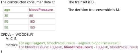
The efficient approach. Notice that Formula 6 above violates the null player property; that is, a variable whose truth value never affects the resulting weight might still receive a nonzero value. For example, the cube 3(¬x2) does not include the variable x5, yet it still affects PDVx5 (since the assignment {x5 = 1, ∀fj̸=5 = 0} satisfies it). As a result, a single cube may influence all the features in the dataset, which significantly hurts WOODELF's performance.
Luckily, Centered Partial Dependence Values (CPDVs), obtained by subtracting the mean prediction on B from each PDV, do satisfy the null player property:
In the WDNF constructed by WOODELF, the mean term 1 |B| ∑b∈B M(b) corresponds to the assignment where all variables are set to 0 (all features are "missing" and taken from B). Combining this insight with Formula 6 yields a simple formula for computing CPDV:
Fig. 4 illustrates how WOODELF++ and Formula 8 compute CPDVs efficiently.
Finally, Formula 9 is equivalent to Formula 8 on WDNFs. It satisfies both linearity and the null player property, making its use within WOODELF both correct and efficient:
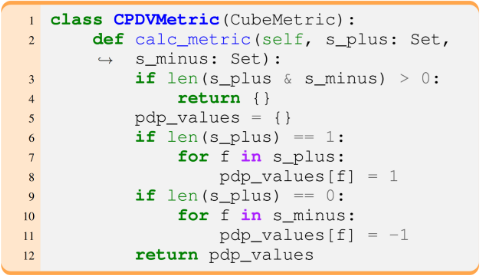
The computation of CPDVs with the WOODELF package is straightforward - Fig. 5 shows the entire code. The computation is performed by calling WOODELF with a CPDVMetric instance, and requires no modifications to the package.
Recovering PDVs from CPDVs is immediate: add back the mean prediction on B. We now present the pseudo-code for our PDP algorithm. Alg. 1 receives a model M, a dataset B, and an integer k, and computes PDPs for all features in B, where each plot uses k sampled points.
A complexity analysis of Alg. 1 is provided in the supplementary material. In short, the WOODELF call (line 3) dominates the runtime: we show that O(vavg c ) = O(vs) = O(D) and that cubes with |S+ k | > 1 can be ignored, leaving only O(2DD) relevant cubes. The complexity is:
Algorithm 1 Efficient Partial Dependence Plot
- 1: function WPDP(M,B, k)
- 2: Select k possible values for each feature in B, and store them in C (see Formula 5).
- 3: CPDV s = WOODELF(M,C,B, CPDVMetric())
- 4: PDV s = CPDV s +M(B).mean()
- 5: Use PDV s to plot the PDP of each feature.
Approximate PDP. Node cover is the number of training samples that reach each node during training. [Friedman, 2001] introduces a PDP approximation based on node cover. [Liu et al., 2025] later observed that this uses the same approximation technique as Path-Dependent SHAP. In cooperative game terms, both methods are defined over the same game. [Liu et al., 2025] also discusses an inconsistency of this approach: it may produce different explanations for functionally equivalent trees.
WOODELF++ leverages this connection to unify approximate and exact PDP under a single algorithm. Specifically, approximate PDP is obtained by computing the same PDV expression on the WDNF built with the Path-Dependent construction. In practice, this reduces to running the algorithm with an empty background dataset, so it defaults to the PathDependent setting (i.e., simply call: WPDP(M, ∅, k)).
The complexity of Alg. 1 with an empty background dataset (see the Path-Dependent complexity in Sect. 2.2):
Approximate PDP : O(kTLD + TL2DD)
4 Full PDP with WOODELF++
Standard PDPs depend on both the number (k) and choice of sampled values. A small k can hide important patterns. For example, a TV-rating model may reveal a sharp viewer spike at lunch (11:30-13:00), but a PDP sampled every four hours (6:00, 10:00, 14:00, 18:00) would miss it.
Some effects are hard to capture even with large k. For instance, a fraud-detection model may learn that users who leave their annual salary at the default value of 60000 are more likely to commit fraud. Even k = 1000 might miss this, as it occurs at a single value within a wide range.
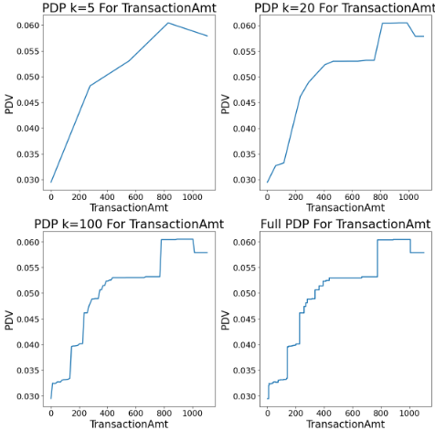
To address this, we introduce Full PDPs, which capture all such behaviors in decision tree ensembles. For a given feature (e.g., age), we take all split thresholds from tree nodes that split on that feature and use them as x-axis values. The rationale is simple: the ensemble changes its prediction only when age crosses one of its thresholds. Between any two consecutive thresholds th1 < th2, the prediction remains constant:
Thus, plotting only these points suffices.
Full PDPs reveal the complete piecewise-constant structure of the decision tree ensemble, including narrow spikes and single-value effects that sampled PDPs often miss. They are particularly useful for detecting overfitting and checking monotonicity. Fig. 6 compares sampled PDPs with different k values to a Full PDP, showing how the latter exactly recovers the true step function using only the feature's split thresholds.
The main drawback is computational cost: large ensembles may have thousands of thresholds per feature. Previously, this made Full PDPs impractical. Both WOODELF++ (via Alg. 1) and FastPD handles large k efficiently, enabling Full PDPs at practical speeds.
5 Any-Order-PDIVs with WOODELF++
In this section, we extend WOODELF to compute all Partial Dependence Interaction Values (PDIVs; see Def. 3). Our approach follows three steps:
- Derive a formula for PDIVs on a WDNF representation.
Figure 7: Python implementation of Formula 11 for a single cube with weight 1. all subsets returns all subsets of a given set.
- Use this formula to implement a Python class inheriting CubeMetric that computes all PDIVs of a cube.
- Run WOODELF with that CubeMetric.
For a pseudo-Boolean function F and variable subset X, PDIV is defined by Formula 10 (combining Def. 2, Def. 3, and Formula 6):
Because PDIV is linear, computing PDIVX on the WDNF reduces to determining the contribution of each cube ck separately and summing the results. We discard unsatisfiable cubes where S+ k ∩ Sk ̸= ∅. A cube affects only subsets X such that S+ k ⊆X ⊆ Sk:
- If X ̸⊆ Sk, the interaction value is zero, since X contains at least one feature that does not appear in the cube and is therefore ignored. Any interaction involving an ignored feature is zero.
- If S+ k ̸⊆X, at least one positive literal is falsified, so all assignments in Formula 10 return zero.
For subsets X where S+ k ⊆ X ⊆ Sk, Formula 10 sums the assignments of all S ⊆ X. The only such S to satisfy the cube and affect the summation is S = S+ k . Thus:
The PDIVMetric code in Fig. 7 uses Formula 11 and computes the effect of a single cube on all relevant subsets X. Running WOODELF++ with PDIVMetric is straightforward:
This simple WOODELF++ call computes all the desired AnyOrder-PDIVs. Here C is used as both consumer and background data, but a separate background dataset can be provided (e.g., using the training set as background). Limiting consumer size is recommended for memory efficiency. An empty background dataset produces approximate PDIVs via the Path-Dependent approach. As WOODELF is GPUfriendly, our method naturally supports GPU acceleration.
This complexity is exponentially better than the previous state of the art, and for balanced decision trees with 2D nodes it becomes polynomial in the input size. A detailed complexity analysis is provided in the supplementary material.
The intuition behind this complexity improvement is as follows. The naive algorithm treats the model as a black box, leading to complexity exponential in the total number of features. FastPD [Liu et al., 2025] improves on this by processing each tree separately; its complexity is exponential in the number of features used per tree, resulting in a worst-case dependence of 22D , which remains exponential in the input size. WOODELF++ advances this line of improvement by treating each root-to-leaf path separately, yielding complexity exponential only in the number of features used per path, i.e., 2D .
6 Joint-PDP with WOODELF++
To compute all Joint PDVs, we use the algorithm from Sect. 5 and the identity:
The algorithm:
- Compute all PDIVs of order 2 and 1 using Sect. 5.
- PDIV{},{} is simply the average prediction on the background data. Compute it directly.
- Apply Formula 12 to obtain PDVs for all feature pairs.
Deriving PDVs from PDIVs, as in Formula 12, is also used in FastPD [Liu et al., 2025]. Since only up to second-order interactions matter, step 1 can ignore cubes with |S+ k | > 2, leaving only O(2DD2 ) cubes to consider.
To construct the consumer dataset, we sample k values per feature. For every pair of features fa and fb, the dataset must contain all k2 value pairs (ai, bj). A naive construction allocates k2 rows per feature, resulting in O(k2 f) rows overall. Specifically, we first construct a size-k consumer data using the PDP procedure (Formula 5). Then, for every feature fa and every sampled value ai, we duplicate the constructed data C and set feature fa to ai in all rows:
Using a more efficient construction (see supplementary material), we reduce the dataset size to only O(k2 log(f)) rows and adapt WOODELF++ to operate on this compressed representation. Overall complexity (see notations in Fig. 3):
This consumer data construction is not specific to WOODELF++. We also use it to accelerate FastPD on Joint-PDP.
As the PDIVs algorithm supports GPU acceleration, JointPDP is also GPU-friendly. Using full PDP sampling, one can plot full Joint-PDPs showing the joint dependence for all values of fa and fb.
7 Experimental Results
The PDP implementation is available in scikit-learn via the partial dependence function. This function implements both the exact method (method='brute') and the approximation method (method='recursion') of PDV computation.
FastPD is implemented in the GLEX R package. It is the current state-of-the-art tool for computing Any-Order-PDIVs. The current implementation focuses on local feature attributions and supports only the case where the background and consumer datasets are identical. We extend the package to support distinct consumer and background datasets. Combined with our consumer-data constructions for PDP, JointPDP, and Full PDP, this enables efficient computation of these tasks within the FastPD framework.
Finally, we implemented WOODELF++ in Python for all discussed tasks and empirically validated it by comparing its outputs to those of scikit-learn.
We compare WOODELF++ running times against scikitlearn and FastPD on two large and widely used datasets:
- The IEEE-CIS fraud detection [kag, 2019] dataset with 472 432 rows and 397 features after one-hot encoding.
- The KDD Cup 1999 intrusion detection [kdd, 1999] dataset with 4898431 rows and 127 features after onehot encoding.
For consistency, these are the same datasets we used in the original WOODELF paper [Nadel and Wettenstein, 2026a]. Additional experiments on smaller datasets and varying tree depths are reported in the supplementary material.
We used scikit-learn's HistGradientBoostingRegressor model, which employs the histogram-based approach popularized by LightGBM [Ke et al., 2017]. In all experiments, models were trained with 100 trees, each limited to a maximum depth of 6, matching XGBoost's widely used default max depth. Experiments were conducted on Google Colab. For CPU training, we enabled the high-memory runtime with 50GB RAM (the default is 12GB). For GPU training, we used the T4 runtime type with high-memory enabled. All experiment notebooks are available in the WOODELFEXPERIMENTS GitHub repository 3 .
As shown in Table 2, our approach outperforms the state of the art, with WOODELF++ achieving a 6× speedup over FastPD on PDP and Joint-PDP. Notably, both FastPD and WOODELF++ significantly outperform scikit-learn, the most widely used tool for this task, with the gap becoming especially pronounced for large k: tasks that take hours or even several days using scikit-learn are completed by both approaches in under 10 minutes.
In Any-Order-PDIVs, where WOODELF++ offers an exponential complexity improvement over FastPD, the preformance gap is substantial. On IEEE-CIS, this improvement translates to a reduction in runtime from an estimated one million years with FastPD to just five minutes using our approach.
3 The WOODELFEXPERIMENTS repository containing all the notebooks used in our experiments: https: //github.com/ron-wettenstein/WoodelfExperiments/tree/main/ woodelf experiments/woodelf pdp/IJCAI26
| IEEE-CIS | ||||
|---|---|---|---|---|
| Task | scikit-learn | FastPD | WOODELF++ | |
| CPU | GPU | |||
| Exact PDP k=5 | 58.5 min | 99 sec | 14.5 sec | 13.1 sec |
| Exact PDP k=10 | 112.4 min | 99 sec | 15.2 sec | 10 sec |
| Exact PDP k=100 | 19 hours* | 99 sec | 14.8 sec | 9 sec |
| Exact full PDP | 59.3 min | 98 sec | 11.8 sec | 7 sec |
| Exact Joint-PDP k=5 | 35 days* | 130 sec | 19 sec | 25 sec |
| Approx. PDP k=5 | 3.3 sec | - | 4.6 sec | 5.4 sec |
| Approx. Joint-PDP k=5 | 19.4 min | - | 10.2 sec | 21.4 sec |
| Any-Order-PDIVs n=10,000 | - | 6·104 years* | 21 sec | 22.6 sec |
| Any-Order-PDIVs | - | 2.9·106 years* | 275 sec | 30.7 sec |
KDD Cup
| Task | scikit-learn | FastPD | WOODELF++ | |
|---|---|---|---|---|
| CPU | GPU | |||
| Exact PDP k=5 | 72.1 min | 520 sec | 95.6 sec | 33.4 sec |
| Exact PDP k=10 | 100.2 min | 519 sec | 95.9 sec | 33.5 sec |
| Exact PDP k=100 | 17 hours* | 519 sec | 96.2 sec | 33.6 sec |
| Exact full PDP | 116.5 min | 519 sec | 90.3 sec | 26.8 sec |
| Exact Joint-PDP k=5 | 9 days* | 568 sec | 95.2 sec | 37.5 sec |
| Approx. PDP k=5 | 5.5 sec | - | 6.5 sec | 8.7 sec |
| Approx. Joint-PDP k=5 | 10.1 min | - | 21.6 sec | 26 sec |
| Any-Order-PDIVs n=10,000 | - | 15 days* | 80.6 sec | 24 sec |
| Any-Order-PDIVs | - | 20 years* | 35 min | 45 sec** |
8 Conclusion
In this work, we extend our previous algorithm, WOODELF, originally designed for Shapley and Banzhaf values, into WOODELF++: a unified framework for efficiently computing PDPs, Joint-PDPs, and Any-Order PDIVs on decision tree ensembles. The two key ideas are to formulate these explanation tasks as linear metrics over WDNF formulas, and to construct compact consumer datasets that allow local-attribution algorithms to efficiently compute global dependence plots. Full PDPs take the latter idea a step further by constructing a consumer dataset that exactly capture the complete piecewise-constant behavior of decision tree ensembles.
This perspective yields substantial computational gains, especially on large datasets. For PDP and Joint-PDP, WOODELF++ is approximately 6× faster than FastPD. For AnyOrder-PDIVs, where WOODELF++ significantly improves the complexity, runtime decrease from several years to just a few minutes.
Acknowledgments
This work was supported in part by the Israel Science Foundation grant 2410/22.
@inproceedings{ijcai2026p562,
  title     = {A Fast and Unified Partial Dependence Plot Algorithm},
  author    = {Wettenstein, Ron and Nadel, Alexander and Boker, Udi},
  booktitle = {Proceedings of the Thirty-Fifth International Joint Conference on
               Artificial Intelligence, {IJCAI-26}},
  publisher = {International Joint Conferences on Artificial Intelligence Organization},
  editor    = {Diego Calvanese},
  pages     = {5048--5056},
  year      = {2026},
  month     = {8},
  note      = {Main Track},
  doi       = {10.24963/ijcai.2026/562},
  url       = {https://doi.org/10.24963/ijcai.2026/562},
}
TY - CPAPER TI - A Fast and Unified Partial Dependence Plot Algorithm AU - Wettenstein, Ron AU - Nadel, Alexander AU - Boker, Udi T2 - Proceedings of the Thirty-Fifth International Joint Conference on Artificial Intelligence, IJCAI-26 PB - International Joint Conferences on Artificial Intelligence Organization PY - 2026 SP - 5048 EP - 5056 DO - 10.24963/ijcai.2026/562 UR - https://doi.org/10.24963/ijcai.2026/562 ER -Copied
Machine-readable versions of this paper, for tools and AI agents:





