Distributed Learning with Adversarial Gradient Perturbations

1 Introduction

Modern learning systems increasingly rely on edge-based architectures, where local devices compute gradient information and communicate it to a central server. In such environments, local gradient reports may be deliberately perturbed to protect sensitive data. This motivates the study of learning algorithms that operate under adversarially corrupted gradients, where each individual gradient reply may deviate arbitrarily from the true gradient, subject only to a known bound on the perturbation magnitude. Understanding what can and cannot be learned in this setting, as well as the query complexity required to do so, is a fundamental question.

Formally, we consider a setting where there are n geographically distributed clients, each holding a convex and Lsmooth loss function ℓi : Rd → R where i ∈ [n]. 1 Define

which is minimized at some w∗ ∈ Rd - when multiple minimizers exist, we define w∗ to be one with the smallest ∥w∗ ∥. 2 The sub-optimality gap of a vector w ∈ Rd is defined as the difference f(w) - f(w∗ ). A server's goal is to find a vector whose sub-optimality gap is bounded by τ > 0.

1 [x] represents the set {1, 2, ..., x} for an integer x ≥ 1.

2 All norms in this paper refer to the L2 norm.

Communication between the server and clients is limited to the following query primitive:

Approximate Gradient Query: The server selects an i ∈ [n] and sends the i-th client a vector w ∈ Rd . The client replies with a vector v satisfying

where ϵ is a value agreed upon in advance by the server and all clients.

Crucially, the client may respond with an arbitrary vector v satisfying (2), including one chosen adversarially so as to impede the server's optimization procedure. Larger values of ϵ expand the set of permissible replies and thus offer stronger privacy protection on the local data contributing to the computation of ∇ℓi(w).

We refer to the above problem as distributed learning with adversarial gradient perturbations (DLAGP). Our goal is to characterize the fundamental feasibility of learning and derive interesting query bounds in this setting. In particular, we aim to answer two questions:

• Q1: How small can the sub-optimality gap be made? Formally, what is the smallest value τmin such that, for all legal inputs {ℓ1, ℓ2, ..., ℓn}, it is possible for the server to find a vector w satisfying f(w) ≤ f(w∗ ) + τmin, possibly using infinitely many queries?
• Q2: Given a value τ that is not "unreasonably small", how many approximate gradient queries are needed for the server to guarantee a sub-optimality gap at most τ?

Our Results and Implications. We establish non-trivial answers to both questions above.

• Answers for Q1 - If no upper bound on ∥w∗ ∥ is known in advance, then no algorithm, even with infinitely many queries, can guarantee finding a vector w with a bounded sub-optimality gap, regardless of the target value τ.

Motivated by this impossibility result, we consider R-instances of the DLAGP problem, where a bound ∥w∗ ∥ ≤ R is known. For this class of instances, we show that the smallest achievable sub-optimality gap τmin lies in the interval [ 1 2 ϵR, 5ϵR]. In other words, when τ < ϵR/2, no algorithm can guarantee a suboptimality gap of τ over all R-instances, even with infinitely many queries. Conversely, the server can always achieve a sub-optimality gap at most τ for all Rinstances whenever τ ≥ 5ϵR.

• Answers for Q2 - For any R-instance satisfying the condition τ ≥ 5ϵR, the server can deterministically ensure a sub-optimality gap at most τ using

queries. For any R-instance satisfying the condition τ ≥ 5.01 · ϵR (the constant 5.01 can be replaced with any value larger than 5), the server can, with probability at least 1 - δ, ensure a sub-optimality gap at most τ using

queries, whereB0 = n

and ˜O(.) hides factors logarithmic to L, R, 1/τ , and 1/δ; note that (4) does not depend on n or d. All queries in this algorithm select clients uniformly at random. By standard sampling arguments, when n is sufficiently large, with high probability each client is queried at most once, and most clients are never queried.

2 RelatedWork

In the study of oracle complexity in convex optimization - an area comprehensively surveyed by [Bubeck, 2015] - the goal is to minimize a convex function f : Rd → R by making the fewest calls to an "oracle". Given a w ∈ Rd , the oracle returns an exact or approximate derivative of f of a specific order at w. For example, an exact zerothorder oracle returns f(w), while a first-order counterpart returns ∇f(w). Our study contributes to the research on firstorder oracles, of which see representative works [Nemirovsky and Yudin, 1983; Tsybakov, 2003; d'Aspremont, 2008; Nemirovski et al., 2009; Agarwal et al., 2012; Dekel et al., 2012; Nesterov, 2012; Jaggi, 2013; Devolder et al., 2014; Kohler and Lucchi, 2017; Lan, 2020; Mirzasoleiman et al., 2020; Huang et al., 2021; Lei and Tang, 2021; Boob et al., 2023; Chai et al., 2023; Garrigos and Gower, 2024; Kerger et al., 2024; Hallak and Levy, 2024] and the references therein.

In the traditional studies of "inexact gradient methods", an approximate first-order oracle returns a stochastically perturbed version of ∇f(w), typically a random ora(w) ∈ Rd whose expectation is ∇f(w). In some cases, there may be a "concentration property" to limit how often ora(w) can deviate from∇f(w) significantly. The seminal work of [Devolder et al., 2014] pioneered the concept of non-stochastic inexact first-order oracles with bounded errors in smooth convex optimization. Our permutation model - formalized as approximate gradient queries (see (2)) - aligns with their concept. Indeed, those queries promise neither expectation nor concentration guarantees, and their answers can be adversarial subject to bounded deviation. This model has gained attention in recent years [Chang et al., 2022; Izzo et al., 2022; Wang and Tan, 2024; Wang and Tan, 2025] - we will discuss the findings of these papers in Section 3.4.

A parallel line of work studies Byzantine-resilient distributed optimization; see, e.g., [Blanchard et al., 2017; Alistarh et al., 2018; Yin et al., 2018; Karimireddy et al., 2021] and the references therein. These works typically assume that most clients return exact or stochastically perturbed gradients, while a fraction of "Byzantine" clients may behave arbitrarily. Algorithms in this literature crucially depend on the existence of sufficiently many honest clients and exploit redundancy through robust aggregation schemes. In contrast, our model does not posit any well-behaved clients: every gradient query may be adversarially perturbed, and no stochastic population-level structure is available. As a result, classical Byzantine-robust techniques do not apply in our scenarios.

Loosely speaking, our work is also related to federated learning, which aims to train models across geographically distributed clients while allowing them to keep data localized; see [Li et al., 2020] for an excellent introduction. A central focus in that area, however, is handling heterogeneous data distributions and ensuring convergence despite differences across client datasets. In contrast, our study abstracts away data heterogeneity and instead examines fundamental limits on learnability, as well as query complexity, under worstcase, bounded adversarial gradient perturbations.

3 Foundation: The Theory with One Client

This section considers DLAGP with only n = 1 client. As we will see Section 4, the theory developed in this section plays a vital role in solving the problem in its general form.

When n = 1, DLAGP can be rephrased in a more succinct manner. Let f : Rd → R be a function such that:

• C1: f is convex and L-smooth;
• C2: f is minimized at some w∗ ∈ Rd ; if multiple minimizers exist, define w∗ to be one with the smallest norm.

The goal of optimization is to find a vector w ∈ Rd whose sub-optimality gap f(w) - f(w∗ ) is bounded by a given τ. The only way for a learner algorithm to glean information about f is to interact with an adversarial gradient perturbation (AGP) oracle. Given a w ∈ Rd , the oracle returns a vector ora(w) ∈ Rd satisfying

where ϵ ≥ 0; we will call it an ϵ-AGP oracle. Our goal is to understand how well and fast optimization can be done when ora(w) can be an arbitrary vector obeying (6).

3.1 No NormBounds, No Call Bounds

We start with a result showing that if nothing is known about ∥w∗ ∥, it is impossible to guarantee a sub-optimality gap τ with a finite number of oracle calls.

Theorem 1. Fix any L ≥ 1, any ϵ ≥ 0, and any τ > 0. If no upper bound on ∥w∗ ∥ is known in advance, no algorithm can guarantee - for every function f : R → R satisfying conditions C1, C2, and ∥∇f(w)∥ ≤ 3τ for all w ∈ R - finding a w ∈ R with f(w) ≤ f(w∗ ) + τ by calling an ϵAGP oracle a finite number of times.

Proof. It suffices to prove the theorem for ϵ = 0 (if ϵ > 0, simply treat a 0-AGP oracle as an ϵ-oracle and apply the argument below). Let us define a function from R to R,

where R > 0 is a real value to be decided later.

As shown in the full version [Sangsiri and Tao, 2026], the function is convex, L-smooth, and ascending. Furthermore, it has the following properties:

• Property 1: minw f(w) = 0, and f(w) = 0 if and only if w ≤ -R.
• Property 2: ∥∇f(w)∥ ≤ 3τ for all w ∈ R, and ∇f(w) = 3τ for all w > -R + 3τ/L.
• Property 3: f(w) ≥ 3τ for any w ≥ -R+ (3τ/L) +1.

Let A be an algorithm that calls a 0-AGP oracle a finite number of calls. We will show that an adversary can force A to incur a sub-optimality gap larger than τ. For this purpose, the adversary initially leaves open the value of R and decides this value only after A has terminated.

Specifically, for any value (i.e., a 1D vector) w that A inquires the oracle with, the adversary always returns 3τ. Let wi be the value that A provides in its i-th call to the oracle, for i ∈ [t] where t is the (finite) number of calls. Let wout be the value output by A. Define

The adversary then sets

which ensures v ≥ -R + (3τ /L) + 1.

The reader can verify that the function f -which is now finalized - has ∇f(w) = 3τ at every w ∈ {w1, w2, ..., wt}. In other words, the oracle's answers to A have been correct. Nevertheless, f(wout) ≥ f(v) ≥ 3τ . Hence, A has failed to ensure f(wout) ≤ f(w∗ ) + τ = τ .

The above argument works only when the adversary does not promise any upper bound on ∥w∗ ∥ in advance. Indeed, ∥w∗ ∥ equals R, which can be arbitrarily big because it depends on the value of v.

3.2 Sub-Optimality Gap

Define

Motivated by Theorem 1, we will study functions from F(R) with a known value of R. Even in this context, learning is still impossible if the target sub-optimality gap is too small:

Theorem 2. Fix any R ≥ 1, any L ≥ 1, and any 0 < ϵ ≤ 1. No algorithm working with an ϵ-AGP oracle can guarantee - for every f ∈ F(R) (recall that the definition of F(R) relies on L due to C2) - returning a w ∈ Rd such that f(w) < f(w∗ )+ϵR/2. This holds true even if the algorithm calls the oracle an infinite number of times.

Proof. Let us define two functions fromR to R:

As shown in the full version [Sangsiri and Tao, 2026]:

• f1 and f2 are convex and L-smooth;
• f1 is ascending and f2 is descending;
• ∥∇f1(w)∥ ≤ ϵ and ∥∇f2(w)∥ ≤ ϵ for all w ∈ R.

Furthermore, the facts below are easy to verify:

• For f1, the optimal vector with the smallest norm is w∗ 1 = -R with f1(w∗ 1 ) = 0, while for f2, the optimal vector with the smallest norm is w∗ 2 = R with f2(w∗ 2 ) = 0. Hence, both f1 and f2 belong to F(R).
• For w ≥ 0, f1(w) ≥ f1(0) = ϵR- ϵ2 /(2L) ≥ ϵR/2.
• For w ≤ 0, f2(w) ≥ f2(0) = ϵR- ϵ2 /(2L) ≥ ϵR/2.

Let A be an algorithm relying on an AGP oracle to minimize f. We observe that A cannot always distinguish between f = f1 and f = f2. Indeed, regardless of f ∈ {f1, f2}, when A solicits ∇f(w) from the oracle, the oracle can always return the value 0, which obeys (6) because ∥∇f(w)∥ ≤ ϵ for both f = f1 and f = f2.

Consider an adversary that is committed to choosing f ∈ {f1, f2} but does so only after A has terminated. Whenever A calls an oracle to inquire ∇f(w), the adversary instructs the oracle to return 0, which is correct no matter f = f1 or f2. Suppose that A finishes by outputting a vector wout. The adversary sets f = f2 if wout ≤ 0, or f = f1 otherwise. This makes sure f(wout) ≥ ϵR/2, forcing the sub-optimality gap to be at least ϵR/2.

3.3 An Optimization Algorithm

Next, we consider f ∈ F(R) and values of τ that are reasonably large. Algorithm 1 describes our optimization algorithm named AGP-opt.

Theorem 3. Let f be a function from F(R). For any real value τ ≥ 5ϵ∥w∗ ∥, algorithm AGP-opt finds a w ∈ Rd satisfying f(w) ≤ f(w∗ ) + τ with parameter

Furthermore, every wk in Line 3 of AGP-opt has norm at most (17/8)R.

Several remarks are in order before delving into the proof:

• Gradient descent (GD) can be regarded as a special instance of AGP-opt with ϵ = 0. The early termination condition at Line 4 is needed to guarantee a suboptimality gap sensitive to ∥w∗ ∥. The sub-optimality gap would become O(ϵR) without early termination, as analyzed in the full version [Sangsiri and Tao, 2026].

Algorithm 1 AGP-opt(K)

• 1: w0 ← 0, k ← 0
• 2: while k < K do
• 3: gk ←ora(wk) /* output of the ϵ-AGP oracle */
• 4: if ∥gk∥ < 4ϵ then return wk
• 5: wk+1 ←wk - 1 2L gk and k ← k + 1
• 6: end while
• 7: return wk

• Theorem 3 extends the convergence bound of GD in a seamless manner: the first term of (10) captures the influence of optimization accuracy, while the second reflects the noise imposed by the ϵ-AGP oracle. For ϵ = 0, the second term disappears, leaving K = 5LR2 /(4τ), which asymptotically matches the convergence bound of GD [Garrigos and Gower, 2024, Corollary 3.5].
• Setting w0 = 0 at Line 1 is needed for the claim (in Theorem 3) that ∥wk∥ ≤ (17/8)R for all k. The claim will be useful in Section 4.2. Our analysis can be easily adapted to other choices of w0 by shifting the origin of the coordinate system to w0.

Proof of Theorem 3. Define

Note that K′ may be less than K - this happens when the termination is at Line 4. The following technical lemma is proved in the full version [Sangsiri and Tao, 2026].

Lemma 4. Let f be a function satisfying C1 and C2. Algorithm AGP-opt outputs a vector w ∈ Rd such that f(w) - f(w∗ ) is bounded by

Furthermore, For any k ∈ [0,K′ - 1], it holds that

As τ ≥ 5ϵ∥w∗ ∥ (a condition in Theorem 3), the value of (12) is at most τ when

The inequality τ ≥ 5ϵ∥w∗ ∥ implies τ - ϵ∥w∗ ∥ ≥ (4/5)τ. Hence,

We can bound from above the right hand side of (15) in two different ways:

where the second inequality used ∥w∗ ∥ ≤ R (because f ∈ F(R))

• On the other hand, from ∥w∗ ∥ ≤ R, we directly have

It now follows from (14) and Lemma 4 that the choice of K in (10) allows AGP-opt to output a w ∈ Rd whose suboptimality gap is at most τ .

For each k ∈ [0,K′ ], Lemma 4 tells us

For the value of K in (10), it holds that k ≤ K′ ≤ K ≤ LR/(4ϵ). Thus, kϵ/(2L) ≤ R/8, from which (16) yields ∥wk - w∗ ∥ ≤ ∥w∗ ∥ + R/8, leading to

This completes the proof of Theorem 3.

3.4 Discussion

Optimization under an ϵ-AGP oracle has been studied in [Chang et al., 2022; Izzo et al., 2022; Wang and Tan, 2024; Wang and Tan, 2025]. We will focus on [Izzo et al., 2022; Wang and Tan, 2024] because the other two papers assume function classes different from ours.

As detailed in the full version [Sangsiri and Tao, 2026], the results of [Izzo et al., 2022] could be used to show that a slightly modified version of GD finds a vector whose suboptimality gap is

where U is an upper bound on f(w) for every vector w produced at any iteration of GD, and B is an upper bound on ∥∇f(w)∥ over those vectors (see the full version [Sangsiri and Tao, 2026] for the precise definitions of U and B). On the other hand, by Lemma 4, we can find a vector whose suboptimality gap is

Our bound (18) converges faster than (17) (specifically: 1/K vs. 1/√K). As K → ∞, our bound converges to O(∥w∗ ∥·ϵ), while (17) to O(∥w∗ ∥ · √Bϵ). Crucially, in the context of [Izzo et al., 2022], a reasonable ϵ must be less than B - otherwise, the fact ∥∇f(w)∥ ≤ B allows an ϵ-AGP oracle to always return vector 0, thereby giving no information to the algorithm at all. In fact, effective optimization demands ϵ ≪ B, in which case our sub-optimality gap O(∥w∗ ∥ · ϵ) is considerably smaller than that of [Izzo et al., 2022].

[Wang and Tan, 2024] presented a mirror-descent algorithm that works when w comes from a domain with a finite radius R. In that scenario, their algorithm ensures a suboptimality gap of

The bound converges slower than (18) (K vs. 1/√K). As K → ∞, (19) converges to O(Rϵ) - note that the bound remains so even if ∥w∗ ∥ ≪ R; in that scenario our bound (18), which converges to O(∥w∗ ∥ϵ), is significantly smaller.

4 DLAGP

We will deploy our theory in Section 3 to tackle the DLAGP problem in its general form (with an arbitrary number n of clients). Every mention of "query" henceforth refers to an approximate gradient query.

4.1 Answers for Q1

Recall that w∗ is an optimal vector of f (i.e., w∗ minimizes the function f defined in (1)) with the smallest norm. If no upper bound is known about ∥w∗ ∥, no DLAGP algorithm can guarantee a sub-optimality gap at most τ using a finite number of queries. Indeed, any such algorithm must work in the special case of n = 1, which, however, gives a contradiction against Theorem 1. This is true even if the values L, ϵ, and τ are all known to the algorithm.

Next, we consider ∥w∗ ∥ ≤ R. Recall (from our statement of Q1 in Section 1) that τmin is the minimum sub-optimality gap that we must tolerate. Theorem 2 implies

To see why, assume the existence of an DLAGP algorithm that can always ensure a sub-optimality gap at most τ for some τ < ϵR/2. Such an algorithm must work in the special case of n = 1, which, however, gives a contradiction against Theorem 2. This is true even if the values ϵ, τ , R, and L are all known to the algorithm.

Next, we argue that τmin ≤ 5ϵR, i.e., DLAGP is solvable on any R-instance as long as τ ≥ 5ϵR. As ℓi is L-smooth for each i ∈ [n], so is the function f in (1). The server only needs to execute the algorithm AGP-opt in Section 3.3. To execute Line 3 of AGP-opt, which demands ora(wk), the server issues a query to every client i ∈ [n], solicits the client's reply vi, and then defines

Accordingly,

which is at most ϵ because ∥vi - ∇ℓi(wk)∥ ≤ ϵ for each i ∈ [n]; see (2). Theorem 3 thus permits the server to ensure a sub-optimality gap at most τ by issuing K ·n queries, where K is given in (10). This yields the bound claimed in (3).

4.2 Answer for Q2

Next, we improve the query bound from the previous subsection when a small failure probability δ is permitted.

Center Estimation. We first take de-tour to discuss a relevant problem. Denote by P = {p1, p2, ..., pn} a set of n vectors in Rd such that ∥pi∥ ≤ B for every i ∈ [n]. Let (s1, s2, ..., sm) be a sequence uniformly sampled from [n]m. Equivalently, each sj (j ∈ [m]) is independently drawn from

[n] uniformly at random. Variations of the following result have appeared before (e.g., Lemma 18 of [Kohler and Lucchi, 2017]); a proof of our version can be found in the full version [Sangsiri and Tao, 2026].

Lemma 5. For any t ≥ 0, by setting m = O((B/t)2 log(1/δ)), we can guarantee

A Randomized Algorithm for DLAGP. Let us return to the DLAGP problem, assuming

Suppose that Line 3 of AGP-opt asks for ora(wk). Instead of querying all clients (as done in Section 4.1), we draw m numbers s1, s2, ..., sm independently from [n] uniformly at random - effectively sampling m clients with replacement. For each j ∈ [m], the server issues a query to solicit a vector vsj from client sj, which comes with the guarantee ∥vsj - ∇ℓsj (wk)∥ ≤ ϵ. Then, it computes

To decide m, we need:

Lemma 6. Suppose that we run AGP-opt by setting K as in (10). For any i ∈ [n] and k ∈ [0,K], it holds that ∥∇ℓi(wk)∥ ≤ B0 + (17/8)LR (see (5) for B0).

The proof can be found in the full version [Sangsiri and Tao, 2026]. From now, we fix B = B0 + (17/8)LR. By Lemma 5, for m= O(( Bt )2 log 1 δ′ ) -where t and δ′ will be decided later - it holds that

Note that 1n ∑ni=1 ∇ℓi(wk) is exactly ∇f(wk). On the other hand, ∥ora(wk) - 1m ∑mj=1 ∇ℓsj (wk)∥, which by (22) is 1m ∥∑mj=1 vsj - ∑mj=1 ∇ℓsj (wk)∥, is no more than ϵ because ∥vsj -∇ℓsj (wk)∥ ≤ ϵ for all j ∈ [m]. Plugging these into (23) gives:

In other words, (22) serves the purpose of a (t + ϵ)-AGP. To apply Theorem 3 and Lemma 6, we require

as ∥w∗ ∥ ≤ R. We therefore set

where the last step used (21).

It remains to fix the value of δ′ . Henceforth, set K = 5LR2 /(4τ); by Theorem 3, AGP-opt performs at most K iterations. By setting δ′ to δ/K, we make sure that the inequality ∥∇f(wk)-ora(wk)∥ ≤ t+ϵ holds for all relevant k with probability at least 1-δ. We thus determine the value of m to be:

where ˜O(.) hides factors logarithmic to L,R, 1/τ, and 1/δ.

We can now conclude that in total m·K queries suffice for the server to guarantee a sub-optimality gap at most τ with probability at least 1 - δ. Plugging in the values of K and m

yields the bound claimed in (4).

5 Experiments

We used three real-world datasets from the LIBSVM library 3 : ijcnn1, covtype, and HIGGS; see the full version [Sangsiri and Tao, 2026]for details on the normalization and cleansing steps taken. Each dataset consists of n pairs (xi, yi) (i ∈ [n]), where xi ∈ Rd is a feature vector and yi ∈ {0, 1} is a binary label. The values of (n, d) for ijcnn1, covtype, and HIGGS are (141691, 22 + 1), (581012, 54 + 1), and (11m, 24 + 1), respectively; see the full version [Sangsiri and Tao, 2026] for the meaning of "+1". Each pair defines a local loss function ℓi(w) where w ∈ Rd . The goal of optimization is to minimize the function f(w) defined in (1). We employed two loss functions for each i ∈ [n]: (i) robust regression (RR), ℓi(w) = (σ(⟨w, xi⟩) - yi)2 , where σ : R → (0, 1) is defined as σ(z) = 1/(1 + e-z ); and (ii) binary cross-entropy (BCE), ℓi(w) = -yi log(σ(⟨w, xi⟩)) - (1 - yi) log(1 - σ(⟨w, xi⟩)). Each ℓi is a convex and Li-smooth function, where the value of Li was calculated based on (xi, yi). The value L (in our problem definition) was determined as maxni=1 Li.

3 Https://www.csie.ntu.edu.tw/∼cjlin/libsvm

Optimization under AGP Oracles. The first set of experiments studies the convergence behavior of the AGP-opt algorithm in Section 3.3. We examined three ϵ-AGP oracles:

• Opposing: the oracle perturbs ∇f(w) by distance ϵ toward the direction opposite to that of ∇f(w);
• Amplifying: the oracle perturbs ∇f(w) by distance ϵ in the same direction as ∇f(w);
• Fixed-Direction: the oracle perturbs ∇f(w) by distance ϵ toward a fixed direction, chosen to be the negative direction of the first dimension of Rd .

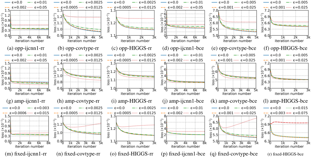
Figure 1 plots the f(wk) value (labeled as "loss" in the diagrams) as a function of k (the current iteration number) for four ϵ values of different magnitudes: ϵ = 0 represents conventional gradient descent, and the other three values form a geometric progression. The caption of each diagram indicates the oracle type, dataset, and local loss functions; e.g., oppijcnn1-rr means that oracle is opposing, the dataset is ijcnn1, and all ℓ1, ℓ2, ..., ℓn adopt the RR function. We disabled the "early termination" condition at Line 4 of AGP-opt. In theory, the condition is needed because when ∥∇f(w)∥ drops to near ϵ, the perturbation of an ϵ-AGP oracle becomes significant and, in the worst case, can be made to harm optimization (as discussed in the full version [Sangsiri and Tao, 2026], the provable sub-optimality gap is higher without such a condition). In practice, however, such worst-case scenarios rarely happen, thus allowing further optimization even beyond the moment of early termination.

The behavior of an opposing oracle in Figures 1(a)-(f) contrasts that of an amplifying oracle in Figures 1(g)-(l). In essence, an opposing oracle suppresses the "step length" of optimization, while an amplifying oracle strengthens it. Under an opposing oracle, higher ϵ values incurred larger suboptimality gaps, but the opposite was observed under an amplifying oracle. This seemingly surprising phenomenon is in fact consistent with the understanding that a step length chosen by theoretical analysis - 1 2L ora(wk) for AGP-opt - is often conservatively small, such that an amplifying oracle "happened to" perform optimization at a better rate.

Figures 1(m)-(r) show that, under a fixed-direction oracle, the red curve - representing a relatively large ϵ value - exhibited a V-shape. To explain why, first note that at the early stages of optimization, the real gradient ∇f(wk) has a large norm such that perturbation has little effect. As the algorithm approaches the optimal vector w∗ , the magnitude of ∥∇f(wk)∥ diminishes, i.e., only small updates are intended. In this case, perturbation dictates the update direction, pulling the algorithm past w∗ and thus causing the loss to go up. Eventually, the optimization converges toward the w where ∇f(w) = (ϵ, 0, 0, ..., 0)T . In fact, for small ϵ values such V-shapes also exist but they are difficult to observe.

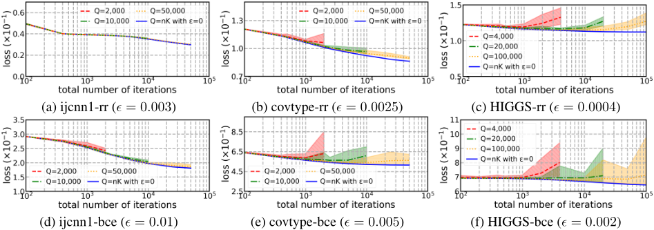
Query Budget Allocation in Distributed Learning. The second set of experiments investigates distributed learning under a specific query budget Q, i.e., the number of queries that the server can afford to issue. We consider that the server allocates the budget as follows. First, it chooses a parameter K ≤ Q, which is the total number of iterations of AGP-opt (without early termination) to perform. Then, in each iteration, it issues m = Q/K queries to compute ora(wk) as in (22). There is a tradeoff: K needs to be sufficiently large for AGP-opt to do enough iterations to approach w∗ , but increasing K reduces m, which elevates the uncertainty in center estimation (see Lemma 5). Our purpose is to provide a guideline for choosing K properly.

Figure 2 plots the final outcome f(wK), the value of f after K iterations of AGP-opt, as a function of K; we will refer to f(wK) as the final loss. The caption under a diagram indicates the dataset, local loss functions, and ϵ value deployed. In these experiments, when queried with w, a client i ∈ [n] perturbs ∇ℓi(w) using one of the three strategies described earlier - opposing, amplifying, or fixed-direction perturbation - with equal probability. Each diagram includes 4

curves: the orange, green, and red curves are obtained with geometrically-increasing values of Q, as well as a blue curve, marked as "Q = nK with ϵ = 0", corresponding to the "unrealistic" method where the server simply queries every client in each iteration and each client performs no perturbation at all. The blue curve serves as a reference for the best achievable final loss at each K. To account for the randomness in the strategy described in Section 4.2, we use shaded regions to report the range of final loss values across multiple runs.

Evidently, K must not be too small: optimization through gradient-based adjustments does require many steps. In Figures 2(a) and 2(d), the best K turned out to be Q, i.e., only one query was issued per iteration. However, this is not representative: in Figures 2(b), 2(c), 2(e), and 2(f), the shaded regions start to grow considerably after Q/K has dropped below a certain threshold. On the other hand, when Q/K ≥ 100, shaded regions are hardly noticeable in all experiments. Furthermore, at the same K, as long as Q/K ≥ 100, increasing Q provided little help in lowering the final loss value. The above observations suggest that m = 100 queries per iteration are adequate for reliable center estimation, because of which K = Q/100 is a robust choice in reality.

6 Conclusions

We have characterized distributed optimization under adversarial gradient perturbations, a setting in which each client's gradient reply to a server query may arbitrarily deviate from the true gradient, subject only to a known distortion bound. Our work addresses two fundamental questions: (i) what level of optimization accuracy can be guaranteed in the presence of such adversarial replies, and (ii) how many gradient queries are sufficient to reach a given accuracy level. We establish sharp feasibility thresholds on achievable accuracy, showing a strict regime in which no algorithm can guarantee meaningful progress, as well as a complementary regime in which reliable optimization is always possible. For the attainable regime, we develop algorithms that provably reach the target accuracy using a bounded number of queries. Future directions include proving tight bounds on the query complexity and extending this framework to richer function classes.