Can Stationary Distributions of Scale-Invariant Neural Networks Be Described by the Thermodynamics of an Ideal Gas?

1 Introduction

The optimization dynamics of deep neural networks remain poorly understood despite their empirical success. A promising approach is to draw inspiration from physics, which studies systems with many degrees of freedom and complex interactions. In particular, thermodynamics has motivated numerous connections to neural networks [Jastrz˛ebski et al., 2017; Chen et al., 2024; Zhang, 2024; Kozyrev, 2025]. In this work, we extend this line of research and propose a framework that relates neural network optimization to thermodynamic systems. Specifically, we interpret stochastic gradient noise as thermal fluctuations and introduce macroscopic thermodynamic variables, like temperature, pressure, and volume, to describe stationary distributions of stochastic gradient descent (SGD). We also connect these variables to training hyperparameters such as learning rate and weight decay.

We focus on scale-invariant neural networks, which resemble common architectures with normalization layers (e.g., BatchNorm [Ioffe and Szegedy, 2015], LayerNorm [Ba et al., 2016]), while remaining theoretically tractable. Theories not accounting for scale invariance would fail to explain phenomena observed in practical training. Unlike prior works that focused on energy, entropy, and temperature, we show that SGD with weight decay on scale-invariant networks naturally introduces pressure and volume, establishing a direct analogy with the ideal gas law. Our main contributions are:

1. We study scale-invariant neural networks under three training protocols: (1) fixed parameter norm, (2) fixed effective learning rate (ELR), and (3) fixed learning rate (LR). For each setting, we derive the corresponding stochastic differential equation (SDE) that governs the dynamics and characterize their stationary distributions.
2. We introduce a thermodynamic framework for analyzing stationary distributions of SGD. Under a simplified isotropic noise model, we establish the thermodynamic analogy rigorously and validate it empirically, revealing a close correspondence with the ideal gas model.
3. We discuss how the ideal gas model generalizes to actual training of scale-invariant neural networks and show that our framework accurately predicts how the entropy of the stationary distribution varies with learning rate and weight decay.

Overall, our framework reveals a deep link between optimization and thermodynamics, providing a physics-based foundation for interpreting neural network training. This insight can inform future work on training hyperparameters, including learning rate scheduling 1 .

2 Background

In this section, we outline the main concepts from thermodynamics and the optimization of scale-invariant neural networks that form the basis of our analogy. For convenience, a complete list of notations is provided in Appendix A. A broader overview of related work is given in Appendix B.

1 Full paper is available at https://arxiv.org/abs/2511.07308

Thermodynamics. Below we summarize the key principles of thermodynamics relevant to our discussion. A more detailed introduction is given in Appendix C.

• T1 A thermodynamic system is described by state variables, including internal energy U (the total energy of all particles in the system), entropy S (a measure of disorder), temperature T , pressure p, and volume V .
• T2 The First Law of Thermodynamics expresses energy conservation: dU = δQ - pdV , where δQ is the infinitesimal heat supplied to the system. The Second Law of Thermodynamics requires dS ≥ δQ/T, implying that systems evolve toward equilibrium, where an appropriate thermodynamic potential is minimized (T4, T5). A reversible process satisfies dS = δQ/T .
• T3 The Gibbs distribution connects thermodynamics with statistical mechanics. At equilibrium, the probability of microstate i with energy Ei is pi ∝ exp(-Ei/T), with the temperature T controlling the distribution's spread. Internal energy and entropy can be expressed as U = Epi [Ei] and S = Epi [- log pi].
• T4 At fixed T and V , the Helmholtz energy F = U -TS is minimized at equilibrium. The Maxwell relation links derivatives of state variables and helps to determine changes in entropy, which is otherwise difficult to measure. In this case, it is given by ( ∂S ∂V )T = ( ∂p ∂T )V 2 .
• T5 At fixed T and p, the Gibbs energy G = U - TS + pV is minimized at equilibrium, with Maxwell relation -( ∂S ∂p )T = ( ∂V ∂T )p .
• T6 An ideal gas is a simplified model neglecting intermolecular interactions. At equilibrium, its state variables satisfy the ideal gas law pV = RT, where R is the gas constant.
• T7 The isochoric and isobaric heat capacities are CV = ( δQ dT )V and Cp = ( δQ dT )p . For an ideal gas, both are constants with Cp -CV = R. In an adiabatic process, defined by δQ = 0, the ideal gas follows pV γ = const with γ = Cp/CV .

Stationary behavior of SGD. In classical optimization theory, SGD differs from full-batch gradient descent: instead of converging to a single stationary point of the loss function, SGD converges to a stationary distribution centered around it. We denote this distribution by ρw(w), where w ∈ Rd are the model parameters. This behavior is driven by the finite learning rate and stochastic gradient estimates, both of which inject noise into the dynamics, analogous to thermal fluctuations and naturally motivating a thermodynamic perspective.

Scale-invariant networks. Modern architectures often include normalization layers that make preceding parameters scale-invariant, i.e., the output of the normalization layer is independent of the parameter norm. We focus on fully scaleinvariant networks, where the whole output of the network does not depend on the parameter norm (i.e., only on the unit direction vector of the weights). The dynamics of the model on the unit sphere (i.e., the loss evolution) is governed by the effective learning rate (ELR), defined as ηeff = η/∥w∥2 , where η is the usual learning rate (LR) used in SGD iterates.

2 ( ∂f ∂x )y denotes the partial derivative of f w.r.t. x under fixed y.

3 Stationary Distributions of SDE

In this section, we start from a stochastic differential equation (SDE) introduced in prior work [Li et al., 2020; Wang and Wang, 2022] that captures the training dynamics of scaleinvariant neural networks. We adapt this SDE to three training protocols of increasing complexity and derive their stationary distributions under an isotropic noise model, introduced below. Although these stationary distributions have been studied previously, we present them in a unified notation and systematize the results across the three protocols.

We begin by introducing several assumptions that enable a theoretical analysis of SGD. First, we approximate the stochastic gradient noise by a Gaussian random vector, a standard assumption in prior work [Jastrz˛ebski et al., 2017; Mandt et al., 2017] naturally leading to an SDE formulation.

Assumption 1 (Gaussian noise). Let L(w) and LB(w) denote the (full-batch) training loss and the loss on a mini-batch B, respectively. Then,

where ε ∼ N(0, Id) and Σw is a spatially dependent covariance matrix of stochastic gradients 3 .

Second, we focus on scale-invariant networks, which induce scale invariance of the loss function.

Assumption 2 (Scale invariance). For any mini-batch B (including the full dataset), the loss satisfies LB(αw) = LB(w) for all α > 0.

Let r = ∥w∥2 and w = w/r. Then L(w) = L(w). As shown in [Li et al., 2020] (Lemmas 3.1 and B.1), the fullbatch gradient and the covariance matrix of a scale-invariant

Next, we assume that the discrete-time dynamics of SGD can be approximated by a continuous-time SDE.

Assumption 3 (SDE approximation). For sufficiently small (effective) learning rate and weight decay coefficient, the SGD dynamics in the weight space are well approximated by the corresponding continuous SDE.

Finally, we introduce a simplified isotropic noise model, which yields explicit stationary distributions of the resulting SDE. A related assumption has been considered in [Jastrz˛ebski et al., 2017; Wang and Wang, 2022].

3 We treat Σw as implicitly dependent on the batch size and therefore do not model the batch size explicitly.

Assumption 4 (Isotropic noise model). The covariance matrix at a unit vector w takes a form Σw = PwΣPw, where Pw = Id-wwT projects onto the tangent subspace orthogonal to w, ensuring the constraints of Eq. 3, and Σ = σ2Id for some σ > 0. Hence, Σw = σ2Pw and Σ1/2 w = σPw.

With these assumptions in place, we analyze three training protocols and present their corresponding discrete dynamics, SDEs, and stationary distributions. In the main text, we report only the expressions characterizing the stationary distributions; detailed derivations are deferred to Appendix D.

SGD on a Fixed Sphere

A natural way to handle scale-invariant parameters is to optimize them directly on their intrinsic domain, a sphere of fixed radius. This can be implemented by projecting the weights onto the sphere after each update [Kodryan et al., 2022; Loshchilov et al., 2025] or by using Riemannian optimization methods [Cho and Lee, 2017]. Here, we consider projected SGD on the sphere Sd-1 (r) with discrete dynamics

where η is the learning rate and Bk is the mini-batch sampled at iteration k. Taking the continuous-time limit of Eq. 4 yields the SDE governing the direction vector Wt:

where Bt denotes standard Brownian motion in Rd and ηeff = η/r2 is the effective learning rate (ELR). While [Wang and Wang, 2022] analyze the Riemannian version of this SDE, we remain with the Euclidean formulation.

Proposition 1 (Fixed sphere). Under Assumptions 1-4, the stationary distribution on the unit sphere ρ∗w of Eq. 5 is

SGD With Fixed ELR

We next allow the radius to evolve and explicitly include weight decay into the dynamics. We consider training with a fixed ELR, which makes the loss dynamics independent of the parameter norm. This is achieved by scaling the learning rate with the squared norm of the parameters, η = ηeff∥wk∥2 . Although less common, such ELR control has been used in practice [Lyle et al., 2024; Ali Mehmeti-Göpel and Wand, 2024], for example to enhance plasticity in reinforcement learning. The discrete update rule is

where λ is the weight decay (WD) coefficient. The corresponding SDE is

Applying Ito's formula separates the dynamics of the direction vector Wt and the radius rt:

Importantly, the radius follows an ordinary differential equation and therefore evolves deterministically. Under the isotropic noise model, Tr ΣWt = σ2 (d-1) is constant. Consequently, the system converges to a stationary distribution for w on the unit sphere and a fixed stationary radius r∗ .

Proposition 2 (Fixed ELR). Under Assumptions 1-4, the stationary distribution ρ∗w on the unit sphere of Eq. 9 and stationary radius r∗ of Eq. 10 are

SGD With Fixed LR

Finally, we consider standard training with a fixed LR. In this case, the dynamics on the unit sphere depends explicitly on the parameter norm. The SGD update is

which corresponds to the SDE

The induced directionWt and radius rt dynamics are

As in the fixed-ELR case, the radius evolves deterministically and converges to a fixed stationary value r∗ .

Proposition 3 (Fixed LR). Under Assumptions 1-4, the stationary distribution ρ∗w of Eq. 15 and stationary radius r∗ of Eq. 16 are

4 Thermodynamic Framework

In this section, we introduce optimization quantities that correspond to thermodynamic state variables in T1. Our framework is based on the stationary distribution of the weights, ρ∗w , which we relate to the thermodynamic Gibbs distribution (T3). This correspondence naturally identifies thermodynamic microstates i with weight vectors w.

We then define the analogues of temperature T, pressure p, and volume V so that the appropriate thermodynamic potential, Helmholtz energy F (T4) or Gibbs energy G (T5), is minimized at stationary. Concretely, we associate T with the noise level through the ELR and gradient variance, V with the radius, and p with the L2 regularization strength. This correspondence reflects an intuition that higher pressure leads to smaller volume, just as stronger weight decay leads to smaller parameter norms. These interpretations are confirmed by explicit minimization of the corresponding potentials.

Microstates and Weights

Under Assumptions 1-4, the stationary distribution ρ∗w is supported on a sphere Sd-1 (r∗ ). The radius r∗ is either predefined (fixed-sphere protocol) or determined by the training hyperparameters (fixed-ELR and fixed-LR protocols). In this setting, the density on Sd-1 (r∗ ) can be expressed in terms of a density on the unit sphere.

Lemma 1. Let ρw be a density on the sphere Sd-1 (r). Then,

where ρw is the corresponding density on the unit sphere. The associated spherical entropy S(ρw) = Eρw [- log ρw(w)] is

with S(ρw) denoting the spherical entropy of ρw.

As a consequence, ρ∗w has the same functional form as ρ∗w and takes the Gibbs form ρ∗w ∝ exp(-L(w)/T) for all three training protocols (Eqs. 6, 11, 17). This mirrors the equilibrium distribution of a thermodynamic system, pi ∝ exp(-Ei/T) (T3), motivating the identifications i ↔ w, Ei ↔ L(w), U ↔ U(ρw) = Eρw [L(w)], and S ↔ S(ρw).

Thermodynamic Potentials

We now define T, p, and V through the requirement that the corresponding potential is minimized at stationary.

Theorem 1 (Helmholtz energy minimization). Under Assumptions 1-4, consider SGD on a fixed sphere with radius r and ELR ηeff. Defining T = ηeffσ2 2 , the Helmholtz energy F = U - TS is minimized at stationary distribution ρw among all distributions on the unit sphere Sd-1 .

Theorem 2 (Gibbs energy minimization). Under Assumptions 1-4, consider SGD with a fixed ELR ηeff (or a fixed LR η) and WD λ. Let T = ηeffσ2 2 (or T = √ ηλσ2 2(d-1) ), p = λ and V = r2 2 . Then, the Gibbs energy G = U - TS + pV is minimized at the stationary distribution ρw among all distributions supported on a sphere Sd-1 (r) with deterministic radius r > 0.

The proofs and a detailed discussion of the choice of p and V are provided in Appendix D. Importantly, the choice of potential follows thermodynamics: F applies when the volume (radius) is fixed, while G applies when the pressure (weight decay coefficient) is fixed. In both cases, the temperature T is set by constant hyperparameters and thus remains fixed. Therefore, our framework offers an alternative thermodynamic description of SGD stationary distributions 4 .

Ideal Gas Law

Remarkably, inserting the definitions of T, p, and V into the stationary radius r∗ (Eq. 12, 18) yields exactly the ideal gas law pV = RT (T6) with R = d-1 2 both for fixed-ELR (Eq. 21) and fixed-LR (Eq. 22) training protocols. A similar expression also holds in the fixed-sphere case if we introduce "effective" weight decay as pressure (see Appendix D.4).

4 Instead of Assumption 3, one may postulate (1) minimization of the potentials at stationary and (2) deterministic radius (while preserving Assumptions 1, 2, 4), and obtain the same stationary distributions without appealing to the SDE.

This correspondence is particularly striking given the very different microscopic assumptions. In statistical mechanics, the ideal gas law assumes non-interacting particles, so the energy of a microstate i decomposes as Ei = ∑j eij, where eij is the energy of particle j. By contrast, the loss L(w) typically exhibits strong parameter coupling and does not admit a decomposition of the form L(w) = ∑j lj(wj). Nevertheless, under scale invariance, the stationary optimization dynamics obey the same equation of state. While such an assumption would be unnatural in physical systems, requiring interactions to depend on angular coordinates rather than distances, it is natural for neural networks and yields the ideal gas law despite strong parameter interactions.

5 Empirical Validation

To support our theoretical framework, we design experiments inspired by the thermodynamic analogy. We focus on tests that do not follow directly from the SDE formulation, providing strong evidence for the thermodynamic perspective.

(V1) Stationary radius. The SDE predicts that r∗ scales as 4√η/λ when training with a fixed LR, and as √ηeff/λ when training with a fixed ELR. Since this prediction follows directly from the SDE (without invoking thermodynamics), it primarily serves as a sanity check. At the same time, it also verifies the ideal gas law (T6) in our analogy.

(V2) Minimizing thermodynamic potentials. Our analogy predicts that stationary distribution of SGD minimizes the appropriate thermodynamic potential. Numerical experiments cannot test minimization over the entire space of distributions ρw and radii r∗ . Instead, we check whether the observed stationary states minimize F or G at least among the distributions induced by different hyperparameter settings.

For example, in fixed LR training, consider a set of hyperparameter configurations H = {(ηi, λi)}hi=1 . For each (ηi, λi), we train the model and measure the corresponding internal energy Ui, entropy Si, and volume Vi. We then verify that for each (η∗ , λ∗ ) ∈ H:

where T ∗ = √ η∗ λ∗ σ2 2(d-1) and p∗ = λ∗ . A similar procedure applies for the settings with a fixed ELR and on a fixed sphere.

(V3) Maxwell relations. Maxwell relations describe how entropy S varies when thermodynamic variables change (T4, T5). In our setting, training with fixed LR corresponds to fixing p and T, so the relevant Maxwell relation is ( ∂S ∂p )T =

( ∂V ∂T )p . In Appendix D.4, we show this is equivalent to

This elegant equation quantifies, how the two hyperparameters influence the stationary entropy. Similar relations for the fixed sphere and fixed ELR protocols are also derived there.

(V4) Adiabatic process. Previously, we interpreted convergence to a stationary distribution as a non-reversible thermodynamic process. Here, we instead view stationary distributions corresponding to different hyperparameters as states of a reversible process. This perspective enables a thermodynamic analysis of how hyperparameters shape the stationary distribution. We focus on the adiabatic process, defined by δQ = 0 (T7). Although heat Q does not appear explicitly in our analogy, it can be inferred from the First Law (T2) as δQ = dU + pdV . This allows us to define the isochoric and isobaric heat capacities, CV and Cp, as in T7. In Appendix D.5, we show that Cp-CV = d-1 2 = R, matching the ideal gas relation. To simulate an adiabatic process, we vary (η, λ) jointly such that pV γ = const, where γ = Cp/CV . For a reversible adiabatic process, dS = δQ/T = 0 (T2), implying constant entropy. Empirically, this predicts that varying hyperparameters along an adiabatic process gives stationary distributions of different shape supported on spheres of different radii but with identical entropy, i.e., overall "disorder."

6 Isotropic Noise Model Experiments

Experimental setup. We start by validating the isotropic noise model through numerical simulation. Here, we show results for fixed LR, while other training protocols are presented in Appendix E.We consider a scale-invariant function L(w) = 1 + µT w ∥w∥ with some fixed µ ∈ Rd , ∥µ∥ = 1 and train it using noisy gradient descent:

with ε ∼ N(0, Id). We select this function because the SDE theory predicts that, at stationarity, the angular distribution follows a Von Mises-Fisher (VMF) form: ρw(w) ∝ exp(-µT w/T). For this distribution, the analytical values of U and S are known (see Appendix E), allowing direct comparison with simulation results. In this setting, we set d = 3.

Entropy estimation. While calculating mean training loss U is straightforward, estimating entropy S is a more complicated task. We rely on the nearest neighbor entropy estimator [Kozachenko and Leonenko, 1987], which requires a sample from the stationary distribution. In Appendix D.6, we present a detailed entropy estimation protocol. In the experiments, we wait until the loss and radius stabilize during the training run. Then, we maintain a queue of 1000 weight vectors sampled every 50 iterations along the training trajectory to reduce correlation between consecutive samples.

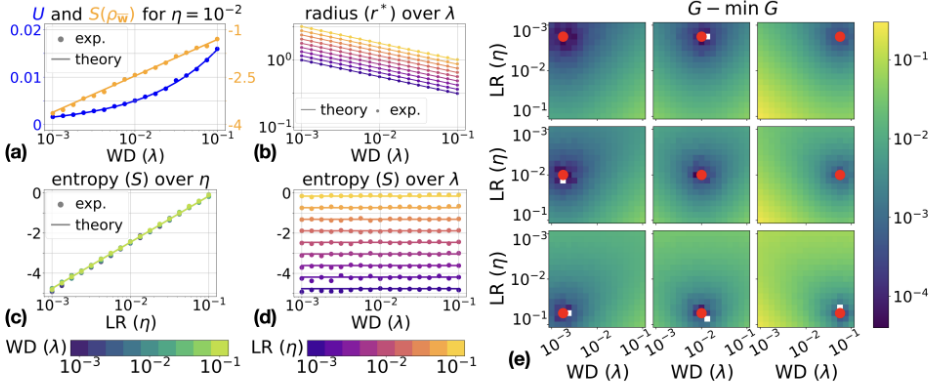
Results. In Figure 1, we present the results of numerical simulation. Subfigure 1a shows that both the average loss U and the entropy on the unit sphere S(ρw) match the analytical VMF predictions, providing a strong evidence, that this distribution is indeed stationary. Subfigures 1b and 1e validate V1 and V2, respectively. To verify V3, we compute the partial derivatives of the total entropy S:

Subfigures 1c,d show that empirical measurements closely follow these theoretic predictions. For V4, we calculate the isochoric heat capacity

Combining it with Cp - CV = d-1 2 , we get γ = Cp CV = 2. In the adiabatic process, we maintain pV γ = const, which reduces to

Therefore, keeping η fixed and varying λ yields an adiabatic process with dS = 0. This is indeed observed in the simulation (Subfigures 1c,d): the entropy depends only on η and remains constant as λ changes. Note that this property is specific to the VMF distribution. For other distributions ρw, the values of CV , Cp, and γ may differ, requiring coordinated changes of η and λ to achieve an adiabatic process.

7 Neural Network Experiments

7.1 Generalizing Isotropic Noise Model

For neural networks, the isotropic noise assumption breaks down: the covariance matrix Σw is generally anisotropic and spatially dependent. [Chaudhari and Soatto, 2018] show that for general networks (i.e., not necessarily scale-invariant) trained with fixed LR η, the stationary distribution takes the form ρ∗w ∝ exp(-Φ(w)/T0) with T0 ∝ η, where Φ(w) is an implicit potential determined by the loss L(w) and the covariance matrix Σw, but independent of η. In this setting, Φ replaces the training loss as the effective energy. An explicit expression for Φ is known only in special cases, such as linear regression [Kunin et al., 2023]. We extend this framework to scale-invariant models by restricting to the unit sphere and defining ρ∗w ∝ exp(-Φ(w)/T0) with T0 determined by training hyperparameters. This distribution arises in all three training protocols introduced in Section 3.

To extend the ideal gas analogy to neural networks, a welldefined stationary radius is required. Following [Li et al., 2020; Wan et al., 2021], we introduce the constant covariance trace assumption, which ensures that Eq. 10 and 16 admit a well-defined limit r∗ .

Assumption 5 (Constant covariance trace). For all w, Tr Σw = const (while the covariance matrix Σw itself might be different). We then define σ2 = 1 d-1 Tr Σw.

Defining T = σ2T0, minimization of Eρw [Φ(w)]-T0S(ρw), achieved at ρ∗w , is equivalent to minimizing

We therefore interpret this quantity as the Helmholtz energy F , minimized in the fixed-sphere case. Consequently, we define G = U(ρw) - TS(ρw) + pV (r), which corresponds to fixed-ELR and fixed-LR cases.

To summarize, the thermodynamic analogy for neural networks differs from the isotropic noise model in two points:

1. The covariance matrix Σw is anisotropic, so the energy function is not the training loss L(w), but a potential σ2Φ(w) with no explicit form.
2. The formulae for temperature T and stationary radius r∗ remain the same as in Section 3, but σ2 = 1 d-1 Tr Σw replaces the isotropic variance.

Thus, under Assumption 5, the ideal gas laws still hold, and we expect the tests V1-V4 to hold. However, since Φ is unknown, we can only directly verify V1 and V3.

7.2 Experimental Setup

We train ResNet-18 [He et al., 2016] on CIFAR10 [Krizhevsky et al., 2009a] with varying LR η and WD λ, fixed batch size B = 128, for t = 106 iterations. The entropy estimation queue stores 1000 vectors with new weights added every 25 iterations. All models are made fully scaleinvariant following [Li and Arora, 2020]. We also use a "thin" model with the width multiplier k = 4 (while the default value is k = 64), the resulting number of trainable parameters is d = 43692. This choice is motivated by (1) memory constraints for storing the entropy estimation queue, and (2) avoiding overparameterization, which imposes a specific behavior of stochastic gradients for small LRs later in training (which advocates convergence to loss minimum, as discussed in Appendix I).In the main text, we show the results only for the fixed LR case, two other training protocols are presented in the Appendix F, supported by the results for the ConvNet architecture from [Kodryan et al., 2022] and the CIFAR-100 dataset [Krizhevsky et al., 2009b]. In Appendix G, we also experiment with partially scale-invariant models.

Estimating entropy in high dimensions is challenging: the nearest-neighbor estimator is unbiased only asymptotically, with a bias of order O(N -2/d ) [Delattre and Fournier, 2017]. We assume the bias is roughly constant across different stationary distributions, allowing accurate reconstruction of entropy derivatives for Maxwell relations. Empirically, V3 holds with high precision, supporting this assumption.

7.3 Results

We present the results in Figure 2. Subfigure 2a shows that σ2 varies across stationary distributions. While theory assumes a fixed σ2 , in practice it depends on the hyperparameters, primarily the product ηλ. We therefore define temperature as T = √ ηλσ2 2(d-1) using the measured σ2 , with values shown in Subfigure 2b. T generally increases with η and λ, but for large λ it can be non-monotonic, e.g., at λ = 10-1 , T decreases for 10-1 ≤ η ≤ 10-0.5 and rises again for η ≥ 10-0.5 , reflecting deviations in σ2 from the trend seen for ηλ < 10-2 . These results suggest that, for large ηλ, stationary distributions explore different regions of the weight space, consistent with prior observations by [Sadrtdinov et al., 2024], who analyze the loss landscape under large LRs.

Subfigure 2c shows that the stationary radius r∗ closely follows theoretical predictions, confirming V1. Deviations appear only at large η and λ, due to discretization error in the SDE: the continuous model neglects the norm of the fullbatch gradient, which acts like a centrifugal force and enlarges r∗ . In Appendix H, we derive a correction that predicts r∗ more accurately for larger values of η and λ.

Finally, to verify V3, we represent S as a function of log η and logλ, as shown in Subfigures 2e and f. The empirical estimates are noisy, so we smooth them using polynomial regression with quadratic terms (see details in Appendix F).

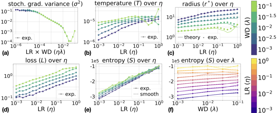
This approximation achieves a coefficient of determination of R2 ≈ 0.99. We then substitute the partial derivatives of the approximation into Eq. 24 and obtain a maximal absolute error of ≈ 3% between the left- and right-hand sides, indicating that the Maxwell relation holds with high precision.

8 Discussion

Extending Ideal Gas Analogy

Answering the question posed in the title, when the assumption TrΣw = const holds, the stationary behavior of SGD is fully consistent with the ideal gas model, as in the isotropic noise setting. In practice, however, we observe that the value of σ2 varies with training hyperparameters. Nevertheless, our experiments show that V1 and V3 remain valid.

Developing a more general thermodynamic description that accounts for variable Tr Σw is an interesting direction for future work. One possibility is to draw an analogy with a real gas, described by the state equation V = Z(p, T) RT p , where Z is the compressibility factor capturing deviations from the ideal gas. This mirrors the relation (r∗ )2 2 = TrΣw ηeff 4λ (from Eq. 10), suggesting that extending the analogy to real gases may be as natural for scale-invariant networks as the ideal gas correspondence established here. Another promising direction is extending the framework beyond fully scale-invariant networks and to more complex optimizers, such as SGD with momentum or Adam [Kingma and Ba, 2015], which could yield insights directly relevant to practical training.

Practical Implications

Our work adopts a thermodynamic perspective to clarify how training hyperparameters, particularly learning rate and weight decay, shape the stationary distribution of SGD. Since neural networks are rarely trained with a fixed learning rate, these insights may inform the design of more effective LR

schedulers [Liu et al., 2025]. A key outcome of our framework is the Maxwell relations, which suggest a possible approach to explicitly control the rate of entropy decay. Properly regulating entropy decay may help reduce training loss while avoiding premature convergence to sharp minima often associated with poor generalization [Kodryan et al., 2022].

Moreover, hyperparameters determine the effective temperature, governing the trade-off between internal energy and entropy. This balance is crucial for weight averaging [Izmailov et al., 2018], which improves performance by combining multiple low-loss checkpoints. While low loss is necessary for accuracy, high entropy promotes diversity of solutions and thus effective averaging, making hyperparameter selection non-trivial. Indeed, [Sadrtdinov et al., 2024] show that LRs optimal for weight averaging often exceed the convergence threshold. Hence, understanding how entropy dynamics affect weight averaging is a promising direction for future work, with Maxwell relations providing a quantitative tool for both theoretical and empirical analysis.

9 Conclusion

In this work, we introduced and empirically validated a thermodynamic framework for describing the stationary distributions of SGD in scale-invariant neural networks. We defined macroscopic thermodynamic variables and related them to learning rate, weight decay, and parameter norm. We rigorously showed that, under the simplified isotropic noise model, stationary distributions follow ideal gas laws. Importantly, the key predictions of this framework also hold in experiments with neural networks. Future work may extend this analogy to settings with variable noise, non-scale-invariant architectures, or more complex optimizers, and may further support principled approaches to hyperparameter tuning for learning rate scheduling and weight averaging.

Acknowledgments

We would like to thank Alexander Shabalin for insightful conversations and personal support. Ekaterina Lobacheva was supported by IVADO and the Canada First Research Excellence Fund. The authors gratefully acknowledge the computing time made available to them on the high-performance computer at the NHR Center of TU Dresden. This center is jointly supported by the Federal Ministry of Research, Technology and Space of Germany and the state governments participating in the NHR (www.nhr-verein.de/unsere-partner). The empirical results were also enabled by compute resources and technical support provided by Mila - Quebec AI Institute (mila.quebec).