The Computational Complexity of Almost Stable Clustering with Penalties

1 Introduction

A fundamental challenge in statistical data analysis is to organize an unlabelled set of data points into groups of similar objects. Clustering, a prominent technique of unsupervised learning, is widely used across various scientific disciplines to address this challenge. The computational complexity of various clustering objectives has been extensively studied in the literature. While many well-known objectives, such as k-Means, k-Median, and k-Centre, are NPhard to optimize [Guha and Khuller, 1999; Vazirani, 2001; Drineas et al., 2004], simple heuristics like local search have long been known to perform effectively on real-world data. This disparity has sparked significant interest in beyond worstcase analysis, aiming to identify structural properties of the input data points that enable heuristic algorithms to produce nearly optimal solutions.

[Bilu and Linial, 2012] first introduced the perturbation resilience condition in the context of max-cut clustering. [Awasthi et al., 2010] studied stables instances of centre-based clustering objectives (including k-MEANS and k-MEDIAN) and proved that 3-stable instances of these problems are solvable in polynomial time. Since then, the challenge has been to determine the smallest stability value for which the problem is in P. [Balcan and Liang, 2016] improved the bound to 1 + √2, and [Makarychev et al., 2012] showed that with a slightly weaker promise of metric perturbation resilience, 2-stable instances of a class of centre-based clustering objectives can be optimized in polynomial time. [Friggstad et al., 2019a] focused on metrics of bounded doubling dimension (which include Rd for constant d) and proved that for any constant ε, (1 + ε)-stable instances of k-MEANS and k-MEANS are solvable in polynomial time. They complemented this result by showing that when the dimension d is part if the input, a universal constant ε◦ exists such that even a PTAS for (1 + ε◦)-stable instances of k-MEANS in Rd would imply NP = RP.

The definition of stable clustering problems is motivated by the intuition that most real-world instances of such problems behave in a "stable" manner for the right objective [Bilu and Linial, 2012], i.e., the structure of the optimum solution is resilient against small perturbations in input values. Here, the objective value of a solution is used as a proxy for its resilience to perturbation, i.e., for stable instances the solution with the optimum objective value must maintain its optimality under a set of valid perturbations. To address cases when this model of stability is too restrictive, the notion of α-stability can be relaxed to ensure that perturbing the metric keeps the optimum solution "β-close" (for some notion of closeness) to the optimum solution of the original metric, for some β ≥ 0. [Ben-David et al., 2006] viewed stability as a property of the clustering algorithm itself, and allowed for various optimum solutions that are structurally similar under Hamming distance. [Balcan and Liang, 2016] introduced (α, β)-stable instances of centre-based clustering (see Section 2 for details) and provided an approximation scheme for (α, β)-stable instances of k-MEDIAN when α > 2 + √3 and β is a function of the minimum size of a cluster in the optimal solution.

1.1 Our Contribution

We study the perturbation resilience of k-MEANS and kMEDIAN in metrics of bounded doubling dimension. Our ultimate goal is to give tight bounds on the (α, β)-stability parameter of efficiently solvable problem instances. While we do not fully close the gap, we make significant progress towards this goal by establishing both upper and lower bounds, thereby providing a more refined picture of the complexity of the problem. Our results also extend to the penalty version of k-MEANS and k-MEDIAN, in which points may not be assigned to a cluster, thus incurring a penalty.

We first consider a special case of (α, β)-stability with β = 0. This notion of stability, which we call strongly α-stable (see Section 2) still generalizes the definition used in recent works, including the one used in [Friggstad et al., 2019a]. We show that such instances of the k-MEANS and k-MEDIAN (with penalties) are solvable over doubling metrics:

Theorem 1 (Exact Solution for Stable k-MEANS). For any given (1+ϵ′ )-stable instance of k-MEANS in doubling metrics, Algorithm 1 finds an optimal solution in polynomial time.

Theorem 2 (Exact Solution for Stable Penalty k-MEANS). Fix any d ≥ 1 and ε′ > 0. (1 + ε′ )-stable instances of the k-MEANS problem in metric spaces with doubling dimension d can be solved in polynomial time.

A PTAS for the Stable k-MEANS problem in doubling dimensions is known in the literature [Friggstad et al., 2019b]. But as noted by [Friggstad et al., 2019a], this result does not imply that the Stable k-MEANS is polynomial-time solvable in doubling dimensions. It is natural to ask if choosing a suitably small error parameter ε for the local search and then using the stability of the optimum solutions together lead to an exact solution. However, this approach may lead to values of ε that are inverse polynomials in n, leading to exponential running times as the local search considers all swaps of size roughly nO(1/ε) .

Next, we focus on the hardness of (α, β)-stable instances (which we call "almost stable" instances). Assuming ETH, we prove that an optimal solution cannot be obtained, even if we allow the algorithm a super-polynomial runtime, and restrict the instance to a bounded-dimensional Euclidean space.

Theorem 3 (Hardness of Almost Stable Penalty k-MEDIAN). For any α ∈ (1, 1.2), β > 0, there is no f(k)no(√k) -time algorithm for (α, β)-stable Euclidean k-MEDIAN with penalties in R2 , unless ETH fails.

Theorem 4 (Hardness of Almost Stable k-MEDIAN). For any α ∈ (1, 1.2), β > 0, there is no f(k)no(√k) -time algorithm for (α, β)-stable k-MEDIAN in metrics of bounded doubling constant, unless ETH fails.

Finally, to complement our algorithmic upper bounds for α-stable instances of k-MEANS/k-MEDIAN (with penalties), we ask the question: how close to one can α get to ensure the instance is still efficiently solvable? While we do not obtain APX-hardness, we manage to show that for inverse polynomial values of ε, the problem is not likely to have an FPT solution.

Theorem 5 (Hardness of (1 + 1 poly(n) )-Stable Penalty k-MEDIAN). There is no f(k)no(k) -time algorithm for (1 + O ( 1 n12 ))-stable Euclidean k-MEDIAN with penalties in R4 , unless ETH fails.

Theorem 6 (Hardness of (1 + 1 poly(n) )-Stable k-MEDIAN). There is no f(k)no(k) -time algorithm for (1+O ( 1 n16 ))-stable Euclidean k-MEDIAN in R6 , unless ETH fails.

Due to page limits, many formal proofs are omitted; the reader is referred to the full version of the paper for more details [Khodamoradi et al., 2025].

2 Preliminaries

Consider a doubling metric space (V, δ), where V is a set of points and δ a distance function over V with doubling dimension d. We focus on stable instances of discrete clustering problems k-MEANS and k-MEDIAN, with and without penalties, over V with metric δ. Let X ⊆ V be a finite set of data points, C ⊆ V to be a finite set of candidate centres, p : X → R a penalty function, δ : V × V → R be a metric, and k be an integer. We denote a k-MEANS/k-MEDIAN instance as a triple (X,C, δ), and a k-MEANS/k-MEDIAN with penalties instance as a four-tuple (X, C, p, δ). A feasible solution to the instance is a set S ⊆ C with |S| = k. For k-MEANS(k-MEDIAN) the cost of solution is defined as cost(S) := ∑j∈X δ(j, S)2 (cost(S) := ∑j∈X δ(j, S)), and for k-MEANS(k-MEDIAN) with penalties the cost of solution is defined as costpen(S) := ∑j∈X min (δ(j, S)2 , p(j)) (costpen(S) := ∑j∈X min (δ(j, S), p(j))) where δ(j, S) denotes mini∈S δ(j, i). Throughout the paper, we refer to n := |C| + |X| as the size of the input, since the computational complexity of the algorithms is primarily determined by how the algorithm scales with the number of data points.

Next, we define α-stable clustering. Intuitively, α-stability for k-MEANS/k-MEDIAN ensures that the optimal solution for a perturbed metric remains optimal for the original metric. We follow the concept of multiplicative stability, first introduced by [Awasthi et al., 2010] and [Bilu and Linial, 2012], but we present a more general version here. Let α ≥ 1. We call an instance I = (X,C, δ) of k-MEANS/kMEDIAN α-stable if for any δ ≤ δ′ ≤ αδ every optimum solution of the k-MEANS/k-MEDIAN (with penalties) instance I ′ = (X, C, δ′ ) is also an optimum solution for I. Similarly, an instance I = (X, C, δ, p) of k-MEANS/k-MEDIAN with penalties is called α-stable if for any δ ≤ δ′ ≤ αδ and any p′ with p ≤ p′ ≤ α2 · p for k-MEANS and p ≤ p′ ≤ α · p for k-MEDIAN, every optimum solution of the k-MEANS/kMEDIAN with penalties instance I ′ = (X, C, δ′ , p′ ) is also an optimum solution for I.

Let cost(S) and cost′ (S) denote the cost of S before and after perturbation. We also study (α, β)-stable instances of k-MEANS and k-MEDIAN, as defined by [Balcan and Liang, 2016]. Recall that in this generalization, β is a measure of proximity between feasible solutions. Various distance metrics can be considered to define β-closeness. We adopt the notion δbij I : (Ck ) × (Ck ) → R≥0 , defined as follows. However, all our results easily extend to other natural notions of distance. For any S1, S2 ⊆ C with |S1| = |S2| = k, define:

We also generalize this notion to clustering with penalties. Let α ≥ 1 and β ≥ 0. We call an instance I = (X,C, δ) (I = (X, C, δ, p)) of k-MEANS/k-MEDIAN with penalties) (α, β)-stable if for any optimum solution O ⊆ C of I, and any optimum solution O′ ⊆ C of the k-MEANS/k-MEDIAN instance (with penalties) I ′ = (X, C, δ′ ) (I ′ = (X, C, δ′ , p′ )), where δ′ is any symmetric function such that δ ≤ δ′ ≤ αδ (and p′ is any function such that p ≤ p′ ≤ α2 ·p for k-MEANS, and p ≤ p′ ≤ α · p for k-MEDIAN), we have δbij I (O,O′ ) ≤ β.

Observe that β = 0 yields the definition of strongly α-stable instances. If β > 0, we call the instance of k-MEANS/kMEDIAN an almost stable instance. Below, we study the performance of a local search algorithm for cases where α is close to 1, that is α = 1+ε′ . To avoid confusion, we use ε′ to refer to the stability parameter, and ε to refer to a parameter of our local search analysis. It should be mentioned that ε only affects the runtime of the local search and is a function of ε′ .

3 Polynomial Algorithms for Stable Clusterings

In this section, we generalize the exact polynomial-time algorithm of [Friggstad et al., 2019a] by incorporating penalties. Most of the results in this section are an adaptation of those in [Friggstad et al., 2019a]. We first show how to obtain optima for k-MEANS without penalties in doubling metrics (see Theorem 1). Doubling metrics are those metrics for which the doubling dimension is a constant. A metric is said to have a doubling dimension of d if every ball of radius R in that metric can be covered with at most 2d balls of radius R/2.

Next, we define a polynomial-time algorithm for k-MEANS with penalties (see Theorem 2). Let (X, C, p, δ) be an instance of k-MEANS with penalties, and Fk = {S ⊆ C : |S| = k} the set of feasible solutions. Throughout this section, we use Algorithm 1, a generalization of the local search method introduced by [Friggstad et al., 2019a] to k-MEANS with penalties. Their original algorithm is the standard ρ-swap local search algorithm, modified to perform the swap that provides the best improvement at each step. We set ρ = dO(d) · ε-O(d/ε) .

Algorithm 1 ρ-Swap Local Search

Input: Let Fk be the family of feasible sets. Let S ∈ Fk. Output: The local optimal set S

• 1: while there exists a set S′ ∈ Fk such that |S -S′ | ≤ ρ and cost(S′ ) < cost(S) (costpen(S′ ) < costpen(S)) do 2: S ← argminS′∈Fk,|S-S′ |≤ρ cost(S′ ) (argminS′∈Fk,|S-S′ |≤ρ costpen(S′ ) )
• 3: end while
• 4: return S

To expand Friggstad et al.'s terminology to the case with penalties, for any S, O ∈ Fk, define:

• For j ∈ X, let σ(j, S) be the centre in S nearest to j, breaking ties by a fixed ordering of C.
• XS,O = {j ∈ X : σ(j, S) ∈ S - O and σ(j,O) ∈ O - S}.
• Xpen S,O = {j ∈ X : σ(j, S) ∈ S-O and σ(j, O) ∈ O-S and δ(j, S)2 , δ(j, O)2 < p(j)}.
• Ψ(S,O) = ∑j∈XS,O δ(j, σ(j, S))2 + δ(j, σ(j,O))2 , Ψpen(S, O) = ∑j∈Xpen S,O δ(j, σ(j, S))2 + δ(j, σ(j, O))2 .

[Friggstad et al., 2019a] first showed that Algorithm 1 visits a "nearly-good" solution in a polynomial number of rounds and returns such a solution upon termination. Next, they used the properties of stable instances to show that any nearlygood solution must be the unique optimal solution, hence Algorithm 1 is an exact polynomial-time algorithm to solve the problem. Adapting their proof to our generalized definition of stability is technically non-trivial. To this end, we begin by modifying the notion of nearly-good solutions.

Definition 1. We call S ∈ Fk a nearly-good solution if for every optimum solution F ∈ Fk we have cost(S) ≤ cost(F )+ 2ε · Ψ(S, F) for k-MEANS and costpen(S) ≤ costpen(O) + 2ε · Ψpen(S, F) for k-MEANS with penalties.

Adapting a technique introduced by [Friggstad et al., 2019b], we can show the existence of a desirable partitioning of the set of centres via a probabilistic argument. Fix any S′ , O′ , T ⊆ C and X′ ⊆ X such that S′ and O′ are disjoint, T ⊆ O′ ∪ S′ , and |T| = |O′ | = |S′ |. Define ∆Tj for each j ∈ X′ to be δ (j, σ (j, S ′△T))2 - δ (j, σ (j, S ′ ))2 . ∆Tj denotes the change in j's assignment cost when solution S′ is replaced by S′∆T . One obtains the following.

Theorem 7 (Theorem 5 in [Friggstad et al., 2019a]). There is a randomized algorithm that samples a partition π of S′ ∪ O′ such that |T ∩ S′ | = |T ∩ O′ | ≤ ρ for each T ∈ π and

Next, we observe that if a feasible solution S is not nearlygood according to our more strict definition, it still holds that the local search algorithmmust take a large step on S:

Theorem 8 (Theorem 6 in [Friggstad et al., 2019a])). For any S,O ∈ Fk, if cost(S) > cost(O) + ε · Ψ(S,O), then there exists an S′ ∈ Fk with |S -S′ | ≤ ρ and cost (S′ ) ≤ cost(S) + ( cost(O) - cost(S) +ε · Ψ(S, O))/k.

With the new definition of nearly-good solutions not being tied to a unique global optimum, we need a more intricate argument to show that local search always makes significant progress towards a nearly-good solution. To that end, we specify, for each set S produced by the algorithm at an iteration, the global optimum which is a witness to S not being nearly-good and show the existence of such a set S is a contradiction.

Lemma 1. Given any instance of the k-MEANS problem, Algorithm 1 with ρ = dO(d) · ε-O(d/ε) terminates at a nearly-good solution. Also, within 2k · ln(n∆) iterations, the algorithm produces a nearly-good solution, where ∆ = maxj∈X,i∈C δ2 (i, j).

3.1 Stable k-MEANS without Penalties

Lemma 1 alone does not guarantee that Algorithm 1 finds an optimal solution for the (1+ε′ )-stable instances of k-MEANS.

We use the stability condition to show that a nearly-good solution must be one of the optimal ones for the instance. Combined with the fact that the returned solution of Algorithm 1 is nearly-good we get the desired result:

Theorem 1 (Exact Solution for Stable k-MEANS). For any given (1+ϵ′ )-stable instance of k-MEANS in doubling metrics, Algorithm 1 finds an optimal solution in polynomial time.

Proof. We need to modify Lemma 2 in [Friggstad et al., 2019a]. We first perturb the distances as follows:

We present a modified version of Lemma 2:

Lemma 2 (Lemma 2 of [Friggstad et al., 2019a], Restatement). If for feasible solutions S,O ∈ Fk, we have that if cost(S) ≤ cost(O) + 2εΦ(S, O), then cost′ (S) ≤ cost′ (O).

In this lemma, we let S be the nearly-good solution of Algorithm 1. Let O be any optimum solution of I ′ . Using stability condition O should also be an optimum solution for I. We observe that cost′ (S) = cost(S) ≤ cost′ (O), where cost′ indicates the cost of a solution under δ′ . Therefore S is a optimum solution for I ′ . Using the stability condition one more time, we conclude that S must also be an optimum solution of I and this S ∈ O = {O1, . . . ,Oℓ}. Assume that Algorithm 1 encounters S in iteration t ≤ ⌊2k · ln(∆n)⌋. Since S has the lowest possible cost for the instance I, the local search must terminate at iteration t and return S.

3.2 Stable k-MEANS with Penalties

We now provide polynomial-time exact ((1 + O (ε′ ))-approximate) solutions for stable instances of k-MEANS with penalties in doubling metrics. All results in this section extend to kMEDIAN with minor modification. We first show how to solve (1 + ε′ )-stable instances of k-MEANS exactly in polynomial time when the metric has a bounded doubling dimension. We first focus on (1 + ε′ )-stable instances for which any optimal solution will remain the optimum for the perturbed instance.

Theorem 2 (Exact Solution for Stable Penalty k-MEANS). Fix any d ≥ 1 and ε′ > 0. (1 + ε′ )-stable instances of the k-MEANS problem in metric spaces with doubling dimension d can be solved in polynomial time.

The local search in [Friggstad et al., 2019a] is oblivious to penalties and cannot guarantee nearly-good solutions under this new setting. Our core idea for addressing this issue is to capture the penalties for the points of X by adding a dummy centre z∗ to V (specifically, to C) and defining C ′ = C∪{z∗ }. We extend δ to V ∪ {z∗ } by setting δ(z∗ , j)2 = δ(j, z ∗ )2 = p(j) for every j ∈ X, and δ(z∗ , c) = 0 for all c ∈ C ′ . Here z∗ is introduced solely to provide the intuition that analyzing the local search algorithm for k-MEANS with penalties is equivalent to analyzing a restricted local search over the reduced k-Means problem where z∗ cannot be swapped. Also note that δ no longer satisfies the triangle inequality, making the analysis more challenging. For any solution S of the k+1-MEANS instance (X,C ′ , δ) that contains z∗ , the cost of S equals the cost of S\{z∗ } for the original k-MEANS with penalties instance (X,C, p, δ). Thus, the task of finding the optimum solution of the (X,C, p, δ) instance is reduced to finding the optimum solution that contains z∗ for the k + 1MEANS instance (X, C ′ , δ). Our key insight here is to modify the ρ-swap algorithm to ensure it always makes the cheapest swap that does not evict z∗ . This eliminates the need to invoke the triangle inequality on z∗ .

We first show that our modified local search converges to a nearly-good solution in polynomial time. Then, we prove that the stability condition ensures that any such nearly-good solution is, in fact, the optimal one. While the structure of our proof is similar to Friggstad et al.'s, we need to tackle challenges in each step. We will highlight how we address these challenges in what follows.

Before rigorously proving Theorem 2, we prove that a nearly-good solution can be found in polynomial time for k-MEANS with penalties as well. To do so, it suffices to replicate Theorem 8 for the penalty setting. Consider the original instance (X, C, p, δ) and fix any S, O ∈ Fk. Define S′ = S\O and O′ = O\S, and fix some T ⊆ O′ ∪ S′ such that |T| = |O′ | = |S′ |. Moreover, for any j ∈ Xpen S,O define ˜∆Tj to be min(δ (j, σ (j, S ′△T))2 , p(j))-δ (j, σ (S ′ ))2 . Using Theorem 7 with X′ = Xpen S,O , there exists a randomized algorithm that samples a partition π of S′ ∪ O′ with |T ∩ S′ | = |T ∩ O′ | ≤ ρ for each T ∈ π such that

The following result extends Theorem 6 of [Friggstad et al., 2019a] to handle penalties, via a more involved case analysis.

Theorem 9. For any S,O ∈ Fk, if costpen(S) > costpen(O) + ε · Ψpen(S,O), then there exists an S′ ∈ Fk with |S - S′ | ≤ ρ such that

Similarly to deriving Lemma 1, we prove the following.

Lemma 3. For k-MEANS with penalties, when Algorithm 1 terminates, the returned solution is nearly-good. Also, for at least one of the first 2k · ln(n∆) iterations of Algorithm 1, S is a nearly-good solution, where ∆ = maxj∈X,i∈C δ2 (i, j).

Proof of Theorem 2 Let ε satisfy 1 + 6ε = (1+ ε′ )2 , i.e., ε ≈ ε′ /3 for small ε′ . Moreover, let S be the nearly-good solution that Algorithm 1 encounters within 2k · ln(n∆) iterations (by Lemma 3). Define a perturbed distance function δ′ as in (2) and a perturbed penalty function via

Moreover, for any S′ ∈ Fk, let cost′pen (S′ ) = ∑j∈X min(mini∈S′ δ′ (i, j)2 , p′ (j)) be the cost of S′ under δ′ . Clearly, δ ≤ δ′ ≤ (1 + ε′ ) · δ and p ≤ p′ ≤ (1 + ε′ )2 · p. Let Oq be any optimum solution w.r.t. cost′pen , due to stability condition O should be an optimum solution w.r.t. costpen. Therefore, S is nearly good for Oq. Partition X as follows:

• X1 = {j ∈ X : σ(j, S) ∈ S - Oq and σ(j,Oq) ∈ S ∩ Oq and δ(j, S)2 < p(j)}
• X2 = {j ∈ X : σ(j, S) ∈ S ∩ Oq and σ(j,Oq) ∈ Oq - S and δ(j, Oq)2 < p(j)}
• X3 = {j ∈ X : σ(j, S), σ(j,Oq) ∈ S ∩ Oq or δ(j, S)2 , δ(j, Oq)2 ≥ p(j)}
• X4 = {j ∈ X : σ(j, S) ∈ S - Oq and σ(j,Oq) ∈ Oq - S and δ(j, S)2 , δ(j, Oq)2 < p(j)}.

Observe that X4 = Xpen S,Oq . As in the proof of Theorem 9, let c∗j = min{δ(j, σ(j,Oq))2 , p(j)} be the cost incurred by point j in the optimum solution, and analogously cj = min{δ(j, σ(j, S))2 , p(j)} for S. To calculate cost′pen (Oq), we consider each j ∈ X case by case. (i) If j ∈ X1 ∪ X4 , then p′ (j) = (1 + ε′ )2p(j) and δ′ (i, j) = (1 + ε′ )δ(i, j) for all i ∈ Oq. Thus, min{mini∈Oq {δ′ (i, j)2 }, p′ (j)} = (1 + ε′ )2 c∗j . (ii) For j ∈ X2 , only i = σ(j, S) ∈ Oq does not have its δ′ (i, j)2 multiplied by (1 + ε′ ). Thus, if δ2 (j, S) ≤ p(j) we have min{mini∈Oq {δ′ (i, j)2 }, p′ (j)} = min{(1+ε′ )2 c∗j , δ(j, S)}. Otherwise, min{mini∈Oq {δ′ (i, j)2 }, p′ (j)} = min{(1 + ε′ )2 c∗j , p(j)}. Hence, min{mini∈Oq δ′ (i, j)2 , p′ (j)} = min{(1 + ε′ )2 c∗j , cj}. (iii) For j ∈ X3 clearly min{mini∈Oq δ′ (i, j)2 , p′ (j)} = cj = c∗j . Thus we derive

Finally, we require Lemma 4.

By Lemma 4, we bound costpen(S) in the following way: costpen(S) ≤ costpen(Oq) + 2ε · Ψpen(S, Oq)

The last bound again uses c∗j ≤ cj for j ∈ X2 . Recall we chose ε so that (1 + 6ε) = (1+ ε′ )2 . Thus, combining Lemma 4, (6) and the simple observation that cost′pen (S) = costpen(S), we get that cost′pen (S) = costpen(S) ≤ cost′pen (Oq). Which means that S is an optimum solution for (X, C, p′ , δ′ ). This completes the proof.

4 Hardness of (α, β)-stable k-MEDIAN

Section 3 discussed steps towards finding optimum and nearoptimum solutions of (α, β)-stable k-MEANS/ k-MEDIAN with or without penalties. Next, we complement this with hardness results for (α, β)-stable k-MEDIAN, as the question of whether we can obtain the exact optimum solution of (α, β)-stable k-MEANS/ k-MEDIAN with penalties efficiently remains open. In Sections 4.1 and 4.2, we obtain hardness results for (α, β)-stable k-MEDIAN, respectively, with and without penalties for any α ∈ (1, 1.2), β > 0. While, for ease of presentation, our hardness results are shown for k-MEDIAN, every result in this section readily extends to k-MEANS.

The results of this section are inspired by a reduction of the GRID TILING INEQUALITY problem to k2 -MEDIAN with penalties, which was introduced by [Cohen-Addad et al., 2018]. We here present our adapted version of the reduction from GRID TILING INEQUALITY to k2 -MEDIAN.

Consider any GRID TILING INEQUALITY problem with integer n and collection S of k2 non-empty sets. We define a Euclidean k2 -MEDIAN instance with penalties similar to the one in Theorem 6.2 of [Cohen-Addad et al., 2018]. Let I(S, n) = (X grid ,C grid , pgrid , δ) denote this instance. Fix ε = O(β/n3 ) for any β > 0. Define a set of data points Xgrid in the region consisting of a square of side length 2k+ε(n-1), where the lower left corner of the square is on the origin (i.e., A = {(x, y) | 0 ≤ x, y ≤ 2k + ε(n - 1)}). They are spaced evenly in a grid G, with two consecutive (horizontal or vertical) data points at distance ε from each other; thus there are Σ = (2k/ε + n)2 data points. Each data point ⃗j has a penalty of pgrid (⃗j) = 1. Thinking of this grid as a discrete approximation of the uniform measure on the square A, we work with the discrete measure µ carried by the data points, where each data point is weighted 1, so that ∫∫A dµ = Σ.

For each set Si,j, we introduce |Si,j| ≤ n2 candidate centres, and let Ci,j denote the set of such candidate centres (note that there are k2 such sets), where Ci,j = {(2i - 1, 2j - 1) + ε(u - 1, v - 1) | (u, v) ∈ Si,j}. Note that the candidate centres are also placed on vertices of G, and that if Si,j has all possible pairs so that Si,j = [n] × [n], then Ci,j precisely forms a subgrid of n2 evenly spaced points in which consecutive points are at distance ε from each other and the lower left point of the subgrid lies at (2i - 1, 2j - 1). The final set of candidate centres is given by C grid = ∪1≤i,j≤kCi,j .

Theorem 10 (Theorem 6.2 of [Cohen-Addad et al., 2018]). There exist a ν ≥ 0, such that the GRID TILING INEQUALITY problem with integer n and collection S has a solution if and only if there exists a solution to I(S, n) with cost at most ν.

Previously, we mentioned that µ approximates the uniform measure. Let us elaborate on what we mean by this. Define, R = [-0.5ε, 2k + ε(n - 0.5)] × [-0.5ε, 2k + ε(n - 0.5)] to be a square with bottom left corner (-0.5ε,-0.5ε) and top right corner (2k + ε(n - 0.5), 2k + ε(n - 0.5)). Denote by uR the uniform probability measure on R and define µ⋆ := Σ · uR. In other words, µ⋆ is a constant measure on R with the property µ⋆ (R) = Σ and µ⋆ (M) = 1 for any unit square M. Notice that for any measurable set D and measurable function f, ε2 ∫∫ fdµ can be viewed as the twodimensional Riemann sum for ∫∫D fdµ⋆ . Therefore, ∫∫D fdµ approximates 1 ε2 ∫∫D fdµ⋆ . The following Lemma will formalize this approximation for two specific f and D that will be used later.

Lemma 5. Fix any ⃗a ∈ C. Define Dr to be the circle with centre ⃗a and radius r ≤ 1. Then

4.1 Stable Euclidean k-MEDIAN with Penalties

We will now prove that for any 1 < α < 1.2, 0 < β (α, β)- stable Euclidean k-MEDIAN with penalties in R2 is hard. The proof idea is to show that I(S, n) is also stable. Since any two centres in any Ci,j for 1 ≤ i, j ≤ k are close, for showing (α, β)-stability it is enough to show that, even if we perturb distances by a constant factor, the optimum solution would be k2 candidate centres each from a Ci,j for i, j ≤ k. Intuitively, this is not hard to see, as the cost of switching from⃗a ∈ Ci,j to another ⃗b ̸= ⃗a ∈ Ci,j is relatively small. Conversely, by adding a centre ⃗c in a cluster Ci′ ,j ′ that currently lacks a centre, we can significantly reduce the costs for points located near ⃗c.

Theorem 3 (Hardness of Almost Stable Penalty k-MEDIAN). For any α ∈ (1, 1.2), β > 0, there is no f(k)no(√k) -time algorithm for (α, β)-stable Euclidean k-MEDIAN with penalties in R2 , unless ETH fails.

Proof. By Theorem 10, it suffices to show that I(S, n) is also (α, β)-stable. Consider any δ ≤ δ′ ≤ α · δ and p ≤ p′ ≤ α · p. Define cost′pen (S) = ∑j∈Xgrid mini∈S {min{δ′ (i, j), p′ (j)}} for every S ⊆ C grid . First we prove that every optimal solution O of the k2 -MEDIAN, (Xgrid ,C grid , δ′ , p′ ) cannot have two centres in a Ci,j for 1 ≤ i, j, ≤ k. Assume that there are 1 ≤ i, j, ≤ k such that there exist ⃗a,⃗b ∈ Ci,j ∩O. By the pigeonhole principle, we have i′ and j ′ , 1 ≤ i′ , j ′ , ≤ k such that Ci′ ,j ′ ∩O = ∅. Let O′ = (O\{⃗a}) ∪ {⃗c} for any ⃗c ∈ Ci′ ,j ′ . We then argue that cost′pen (O′ ) is smaller than cost′pen (O), which is a contradiction. Let D be the set of all points in a circle with centre ⃗c and radius 1α . Every ⃗x ∈ D satisfies δ′ (⃗x,⃗c) ≤ αδ(⃗x,⃗c) ≤ 1. Also, since every other point ⃗ d ̸= ⃗a, ⃗ d ∈ O′ , has the property δ(⃗c, ⃗ d) ≥ 2 - (n - 1)ε, we have δ′ ( ⃗ d, ⃗x) ≥ δ(⃗ d, ⃗x) ≥ 2 - α - (n - 1)ε which is greater than 1 for large enough n (for n polynomial in 1 α-1 ). Also, p′ (⃗x) ≥ pgrid (⃗x) = 1 which is smaller than δ′ (⃗x,⃗c). Therefore, every point in D will be assigned to ⃗c. Thus, adding ⃗c to O will decrease cost′pen (O) at least by

where (i) is due to Lemma 5. For any ⃗x ∈ A to be assigned to ⃗a, δ′ (⃗x,⃗a) should be less than p′ (⃗x) ≤ α. Subsequently, all such ⃗x should have δ(⃗x,⃗a) ≤ α, i.e., they should belong to a circle D′ with radius α and centre ⃗a. Also note

Thus, removing ⃗a from O will decrease cost′pen (O) by at most

cost′pen (O′ )-cost′pen (O)≤ 1 ε2 ((α4 -α3 ) 2π 3 - π 3α2 +O(nε)) follows from (7). The latter is less than zero for α ∈ (1, 1.2) for large enough n. This contradicts O minimizing cost′pen .

Consider O′ ∈ Fk2 to be any optimum solution of I(S, n). We have established that O contains k2 centres, one in each Ci,j for 1 ≤ i, j,≤ k. Hence O′ has the same property. Let f : O′ → O be the unique function such that for any o ∈ O′ , if o ∈ Ci,j for some 1 ≤ i, j,≤ k, then also f(o) ∈ Ci,j . Therefore, ∑o∈Op δ(o, fp(o)) ≤ k2 ε(n - 1) ≤ β. So δbij I (O,O′ ) ≤ β. Thus, I(S, n) is (α, β)-stable.

4.2 Stable k-MEDIAN in DoublingMetrics

Focusing on the setting without penalties, we prove that (α, β)- stable k-MEDIAN with doubling constant 8 is hard, for any 1 < α < 1.2, 0 < β. The main proof idea for the following theorem is that while the point set is located in R3 , introducing a metric δpen with doubling dimension 3 (different from standard norm two metric) allows us to replicate the effect of penalties.

Theorem 4 (Hardness of Almost Stable k-MEDIAN). For any α ∈ (1, 1.2), β > 0, there is no f(k)no(√k) -time algorithm for (α, β)-stable k-MEDIAN in metrics of bounded doubling constant, unless ETH fails.

5 Hardness of α-stable k-MEDIAN in Bounded-Dimensional Metrics

[Friggstad et al., 2019a] set out to resolve the complexity of (1 + ε)-stable instances of k-MEDIAN and k-MEANS for constant values of ε, which is highly desirable since this is the range where the ρ-swap local search can produce solutions in polynomial time. However, the computational complexity of the problem remains unknown when we go beyond constant error values. This question is of particular interest when discussing Fixed Parameter Tractable (FPT) algorithms that allow us slightly super-polynomial running times. Therefore, we examine the computational complexity of (1 + ε)-stable instances of k-MEDIAN (and k-MEANS) when ε is an inverse polynomial in n. As the main result of this section, we show that for ε = 1 poly(n) , the problem is still hard.

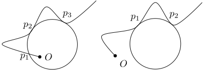
Inspired by [Cohen-Addad et al., 2018], our general approach is to reduce PVC to k-MEDIAN using moment curves. We first establish some useful properties regarding moment curves and spheres. These properties resemble those shown in Section 2.1 of [Cohen-Addad et al., 2018], but are modified to our purpose. The proofs, in particular, utilize Descartes' rule of signs (see [Curtiss, 1918]).

Lemma 6. Let 0 < t1 < t2 < t3. Consider the 4-dimensional moment curve (t, t2 , t3 , t4 ) and the 3-sphere in R4 that goes through the moment curve at t = t1 and is tangent to the curve at t = t2, t3. The segments on the moment curve for t ∈ (t1, t2) ∪ (t2, t3) ∪ (t3,∞) all lie outside of the sphere.

Lemma 7. Let 0 < t1 < t2. Consider the 3-dimensional moment curve (t, t2 , t3 ) and the unique 2-sphere in R3 that is tangent to the moment curve at t = t1, t2. The sphere only touches the curve at t1 and t2.

5.1 (1+ 1 poly(n) )-Stable Euclidean k-MEDIAN with Penalties

This subsection establishes the hardness of (1 + 1/poly(n))- stable Euclidean k-MEDIAN with penalties in R4 . Like [Cohen-Addad et al., 2018], we reduce from PARTIAL VERTEX COVER (PVC) by creating a candidate centre on a moment curve for each vertex of the input graph, along with a data point for each edge of the input graph G = (V, E). For each edge, we ensure that the point corresponding to that edge is closer to the two centres representing each vertex of the edge than to any other candidate centre. This allows us to reduce a PVC instance to a k-MEDIAN instance.

However, to ensure the stability of k-MEDIAN with penalties, we need to guarantee that the difference between the distances of the representation of an edge to its corresponding vertex and to the representation of other vertices is significant.

Moreover, with the reduction introduced by [Cohen-Addad et al., 2018], perturbing the metric function risks having the optimum solution switch from one maximal partial cover of the graph to another. To avoid this, we ensure that the distance between the representation of edges and the representation of their respective vertices remains constant.

Theorem 5 (Hardness of (1 + 1 poly(n) )-Stable Penalty k-MEDIAN). There is no f(k)no(k) -time algorithm for (1 + O ( 1 n12 ))-stable Euclidean k-MEDIAN with penalties in R4 , unless ETH fails.

5.2 (1+ 1 poly(n) )-Stable Euclidean k-MEDIAN

Finally, we focus on k-MEDIAN without penalties and show that (1+ 1 poly(n) )-stable Euclidean k-MEDIAN in R6 is hard. The proof is non-trivial and builds on similar ideas as the proof of Theorem 5.

Theorem 6 (Hardness of (1 + 1 poly(n) )-Stable k-MEDIAN). There is no f(k)no(k) -time algorithm for (1+O ( 1 n16 ))-stable Euclidean k-MEDIAN in R6 , unless ETH fails.

6 Conclusion

This paper addresses the complexity of stable instances of k-MEANS and k-MEDIAN under generalized stability notions, and in the generalized setting with penalties. For our most general stability notion, i.e., (α, β)-stability, the problem is proven highly intractable, even in small-dimensional Euclidean spaces. Some of our proofs build on proof ideas from the related literature; yet they require new and non-trivial technical insights in order to address our generalized settings. We fall short of answering the following question.

• Open Problem 1: Does a PTAS (a (1+ε)-approximation for any constant ε > 0) exist for almost stable instances of k-MEANS/k-MEDIAN?

We conjecture that the answer is yes, as there is evidence that the local search may be producing feasible solutions that are simultaneously near optimal and β-close to one optimal solution. For instance, one can show that the algorithm visits at least one nearly-good solution in a polynomial number of iterations. We also prove that (1 + ε)-stable instances of the problems are solvable in polynomial time, while the (1 + ε)- stable instances are intractable again for inverse polynomial values of ε. Our analysis leaves the following question open:

• Open Problem 2: What is the parameterized complexity of the (1+1/poly(n))-stable instances?

Acknowledgments

K. Khodamoradi was supported by a Natural Sciences and Engineering Research Council (NSERC) Discovery Grant (application no. RGPIN-2024-06360). S. Zilles was supported by a Canada CIFAR AI Chair (held at Amii), an NSERC Canada Research Chair, an NSERC Discovery Grant (application no. RGPIN-2017-05336), and through the New Frontiers in Research Fund under grant no. NFRFE-2023-00109.