
ConDyGNet: Constraint-Guided Dynamic Graph Networks for Multivariate Time Series Forecasting
Proceedings of the Thirty-Fifth International Joint Conference on Artificial Intelligence. Main Track. Pages 4536-4544.
https://doi.org/10.24963/ijcai.2026/505
Keywords
- Machine Learning: Time series and data streams
- Machine Learning: Sequence and graph learning
- Data Mining: Mining data streams
Abstract
Modeling inter-channel dependencies is important for multivariate time series forecasting (MTSF). However, in many cases, inter-channel dependencies are time-varying and subject to noise interference, making it difficult for models to find a balance between structural stability and temporal adaptivity. Existing methods either use a single global static structure, resulting in insufficient sensitivity to temporal changes, or use local statistical correlations to construct dependencies, but local correlations are prone to introducing noise, which may further amplify the impact of noise during propagation. To address these issues, we propose a Constraint-Guided Dynamic Graph Network (ConDyGNet), whose core idea is "global basis, dynamic weights". Specifically, ConDyGNet learns a low-rank global basis as a shared structural constraint and generates patch-wise basis mixing weights to construct dynamic propagation graphs. This maintains topological consistency while allowing local adaptation and reducing the influence of local noise. We conducted extensive experiments on eight public benchmark datasets and multiple forecasting horizons, demonstrating that ConDyGNet can learn more robust time-varying inter-channel dependencies and achieve state-of-the-art forecasting accuracy. The code is available at https://github.com/constli67/ConDyGNet.
- [Abu-El-Haija et al., 2019] Sami Abu-El-Haija, Bryan Per- ozzi, Amol Kapoor, Nazanin Alipourfard, Kristina Ler- man, Hrayr Harutyunyan, Greg Ver Steeg, and Aram Gal- styan. Mixhop: Higher-order graph convolutional archi- tectures via sparsified neighborhood mixing. In inter- national conference on machine learning, pages 21-29. PMLR, 2019.
- [Bai et al., 2020] Lei Bai, Lina Yao, Can Li, Xianzhi Wang, and Can Wang. Adaptive graph convolutional recurrent network for traffic forecasting. Advances in neural infor- mation processing systems, 33:17804-17815, 2020.
- [Cai et al., 2024] Wanlin Cai, Yuxuan Liang, Xianggen Liu, Jianshuai Feng, and Yuankai Wu. Msgnet: Learning multi- scale inter-series correlations for multivariate time series forecasting. In Proceedings of the AAAI conference on ar- tificial intelligence, volume 38, pages 11141-11149, 2024.
- [Cao et al., 2025] Lingxiao Cao, Bin Wang, Guiyuan Jiang, Yanwei Yu, and Junyu Dong. Spatiotemporal-aware trend- seasonality decomposition network for traffic flow fore- casting. In Proceedings of the AAAI Conference on Artifi- cial Intelligence, volume 39, pages 11463-11471, 2025.
- [Chen et al., 2024a] Jialin Chen, Jan Eric Lenssen, Aosong Feng, Weihua Hu, Matthias Fey, Leandros Tassiulas, Jure Leskovec, and Rex Ying. From similarity to superiority: Channel clustering for time series forecasting. Advances in Neural Information Processing Systems, 37:130635- 130663, 2024.
- [Chen et al., 2024b] Xiaodan Chen, Xiucheng Li, Xinyang Chen, and Zhijun Li. Structured matrix basis for multi- variate time series forecasting with interpretable dynam- ics. Advances in Neural Information Processing Systems, 37:24326-24349, 2024.
- [Cini et al., 2023] Andrea Cini, Ivan Marisca, Filippo Maria Bianchi, and Cesare Alippi. Scalable spatiotemporal graph neural networks. In Proceedings of the AAAI conference on artificial intelligence, volume 37, pages 7218-7226, 2023.
- [Das et al., 2023] Abhimanyu Das, Weihao Kong, Andrew Leach, Shaan Mathur, Rajat Sen, and Rose Yu. Long-term forecasting with tide: Time-series dense encoder. arXiv preprint arXiv:2304.08424, 2023.
- [Fischer and Krauss, 2018] Thomas Fischer and Christopher Krauss. Deep learning with long short-term memory net- works for financial market predictions. European journal of operational research, 270(2):654-669, 2018.
- [Han et al., 2024] Lu Han, Xu-Yang Chen, Han-Jia Ye, and De-Chuan Zhan. Softs: Efficient multivariate time series forecasting with series-core fusion. Advances in Neural Information Processing Systems, 37:64145-64175, 2024.
- [Hu et al., 2025] Yifan Hu, Guibin Zhang, Peiyuan Liu, Disen Lan, Naiqi Li, Dawei Cheng, Tao Dai, Shu-Tao Xia, and Shirui Pan. Timefilter: Patch-specific spatial-temporal graph filtration for time series forecasting. In ICML, 2025.
- [Huang et al., 2023] Qihe Huang, Lei Shen, Ruixin Zhang, Shouhong Ding, Binwu Wang, Zhengyang Zhou, and Yang Wang. Crossgnn: Confronting noisy multivariate time series via cross interaction refinement. Advances in Neural Information Processing Systems, 36:46885-46902, 2023.
- [Li et al., 2018] Yaguang Li, Rose Yu, Cyrus Shahabi, and Yan Liu. Diffusion convolutional recurrent neural net- work: Data-driven traffic forecasting. In ICLR (Poster), 2018.
- [Li et al., 2023] Zhuo Lin Li, Gao Wei Zhang, Jie Yu, and Ling Yu Xu. Dynamic graph structure learning for mul- tivariate time series forecasting. Pattern Recognition, 138:109423, 2023.
- [Lin et al., 2023] Shengsheng Lin, Weiwei Lin, Wentai Wu, Feiyu Zhao, Ruichao Mo, and Haotong Zhang. Segrnn: Segment recurrent neural network for long-term time se- ries forecasting. arXiv preprint arXiv:2308.11200, 2023.
- [Lin et al., 2025] Shengsheng Lin, Haojun Chen, Haijie Wu, Chunyun Qiu, and Weiwei Lin. Temporal query network for efficient multivariate time series forecasting. In Inter- national Conference on Machine Learning, pages 37797- 37814. PMLR, 2025.
- [Liu et al., 2024] Yong Liu, Tengge Hu, Haoran Zhang, Haixu Wu, Shiyu Wang, Lintao Ma, and Mingsheng Long. itransformer: Inverted transformers are effective for time series forecasting. In ICLR, 2024.
- [Liu et al., 2025] Peiyuan Liu, Beiliang Wu, Yifan Hu, Naiqi Li, Tao Dai, Jigang Bao, and Shu-Tao Xia. Timebridge: Non-stationarity matters for long-term time series fore- casting. In ICML, 2025.
- [Luo and Wang, 2024] Donghao Luo and Xue Wang. Mod- erntcn: A modern pure convolution structure for general time series analysis. In ICLR, 2024.
- [Meng et al., 2024] Fanyue Meng, Zhaoyuan Lu, Xiang Li, Wei Han, Jieyang Peng, Xiufeng Liu, and Zhibin Niu. Demand-side energy management reimagined: A compre- hensive literature analysis leveraging large language mod- els. Energy, 291:130303, 2024.
- [Nie et al., 2023] Yuqi Nie, Nam H. Nguyen, Phanwadee Sinthong, and Jayant Kalagnanam. A time series is worth 64 words: Long-term forecasting with transformers. In ICLR, 2023.
- [Qiu et al., 2025] Xiangfei Qiu, Xingjian Wu, Yan Lin, Chenjuan Guo, Jilin Hu, and Bin Yang. Duet: Dual cluster- ing enhanced multivariate time series forecasting. In Pro- ceedings of the 31st ACM SIGKDD Conference on Knowl- edge Discovery and Data Mining V. 1, pages 1185-1196, 2025.
- [Schirmer et al., 2022] Mona Schirmer, Mazin Eltayeb, Ste- fan Lessmann, and Maja Rudolph. Modeling irregular time series with continuous recurrent units. In Inter- national conference on machine learning, pages 19388- 19405.
- PMLR, 2022.
- [Shu et al., 2021] Wanneng Shu, Ken Cai, and Neal Naixue Xiong. A short-term traffic flow prediction model based on an improved gate recurrent unit neural network. IEEE Transactions on Intelligent Transportation Systems, 23(9):16654-16665, 2021.
- [Volkovs et al., 2023] Kristofers Volkovs, Evalds Urtans, and Vairis Caune. Primed unet-lstm for weather forecast- ing. In Proceedings of the 2023 7th International Confer- ence on Advances in Artificial Intelligence, pages 13-17, 2023.
- [Wang et al., 2024] Yuxuan Wang, Haixu Wu, Jiaxiang Dong, Guo Qin, Haoran Zhang, Yong Liu, Yunzhong Qiu, Jianmin Wang, and Mingsheng Long. Timexer: Empow- ering transformers for time series forecasting with exoge- nous variables. Advances in Neural Information Process- ing Systems, 37:469-498, 2024.
- [Wang et al., 2025] Chao-fan Wang, Kui-xing Liu, Jieyang Peng, Xiang Li, Xiu-feng Liu, Jia-wan Zhang, and Zhi-bin Niu. High-precision energy consumption forecasting for large office building using a signal decomposition-based deep learning approach. Energy, 314:133964, 2025.
- [Wu et al., 2019] Zonghan Wu, Shirui Pan, Guodong Long, Jing Jiang, and Chengqi Zhang. Graph wavenet for deep spatial-temporal graph modeling. arXiv preprint arXiv:1906.00121, 2019. IJCAI
- [Wu et al., 2020] Zonghan Wu, Shirui Pan, Guodong Long, Jing Jiang, Xiaojun Chang, and Chengqi Zhang. Con- necting the dots: Multivariate time series forecasting with graph neural networks. In Proceedings of the 26th ACM SIGKDD international conference on knowledge discov- ery & data mining, pages 753-763, 2020.
- [Wu et al., 2023] Haixu Wu, Tengge Hu, Yong Liu, Hang Zhou, Jianmin Wang, and Mingsheng Long. Timesnet: Temporal 2d-variation modeling for general time series analysis. In ICLR, 2023.
- [Yi et al., 2023] Kun Yi, Qi Zhang, Wei Fan, Hui He, Liang Hu, Pengyang Wang, Ning An, Longbing Cao, and Zhen- dong Niu. Fouriergnn: Rethinking multivariate time series forecasting from a pure graph perspective. Advances in neural information processing systems, 36:69638-69660, 2023.
- [Yu et al., 2017] Bing Yu, Haoteng Yin, and Zhanxing Zhu. Spatio-temporal graph convolutional networks: A deep learning framework for traffic forecasting. arXiv preprint arXiv:1709.04875, 2017. IJCAI
- [Zeng et al., 2023] Ailing Zeng, Muxi Chen, Lei Zhang, and Qiang Xu. Are transformers effective for time series fore- casting? In AAAI, pages 11121-11128, 2023.
- [Zhang and Yan, 2023] Yunhao Zhang and Junchi Yan. Crossformer: Transformer utilizing cross-dimension de- pendency for multivariate time series forecasting. In ICLR, 2023.
- [Zhao et al., 2023] Kai Zhao, Chenjuan Guo, Yunyao Cheng, Peng Han, Miao Zhang, and Bin Yang. Multiple time series forecasting with dynamic graph modeling. Pro- ceedings of the VLDB Endowment, 17(4):753-765, 2023.
- [Zhou et al., 2021] Haoyi Zhou, Shanghang Zhang, Jieqi Peng, Shuai Zhang, Jianxin Li, Hui Xiong, and Wan- cai Zhang. Informer: Beyond efficient transformer for long sequence time-series forecasting. In Proceedings of the AAAI conference on artificial intelligence, volume 35, pages 11106-11115, 2021.
- [Zhou et al., 2022] Tian Zhou, Ziqing Ma, Qingsong Wen, Xue Wang, Liang Sun, and Rong Jin. Fedformer: Fre- quency enhanced decomposed transformer for long-term series forecasting. In International conference on machine learning, pages 27268-27286. PMLR, 2022.
- [Zhu et al., 2024] Peng Zhu, Yuante Li, Yifan Hu, Qinyuan Liu, Dawei Cheng, and Yuqi Liang. Lsr-igru: Stock trend prediction based on long short-term relationships and im- proved gru. In Proceedings of the 33rd ACM International Conference on Information and Knowledge Management, pages 5135-5142, 2024.
References were extracted automatically from the PDF and may contain errors.
Full text extracted automatically from the PDF; figures, tables and equations may differ. The PDF is the version of record.
1 Introduction
Multivariate time series forecasting (MTSF) is challenging because it requires simultaneously modeling dependencies along both the temporal dimension and between channels. MTSF has wide applications, including traffic flow forecasting [Shu et al., 2021; Cao et al., 2025], weather monitoring [Volkovs et al., 2023], energy analytics [Meng et al., 2024; Wang et al., 2025], and financial investment [Fischer and Krauss, 2018; Zhu et al., 2024]. In recent years, deep learning has facilitated the rapid development of time series forecasting. Recurrent neural networks (RNNs) [Schirmer et al.,
* Corresponding author: Zhibin Niu.
2022], temporal convolutional networks (TCNs) [Luo and Wang, 2024], and Transformer-based models [Zhou et al., 2022; Nie et al., 2023] have demonstrated excellent abilities to learn dynamic changes along the temporal dimension.
Meanwhile, if we view multivariate time series as graph signals, we gain a complementary new perspective: each variable can be seen as a node in the graph, connected by underlying dependencies. This suggests that modeling the relationships between variables is equally important. Based on this, one line of work employs an explicit structure, first learning the dependency graph between variables and then aggregating information through message passing mechanisms [Wu et al., 2020; Cai et al., 2024]. Another line of work relies on implicit interactions, such as channel-wise attention or hybrid modules, to fuse information between variables [Liu et al., 2024; Wang et al., 2024].
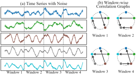
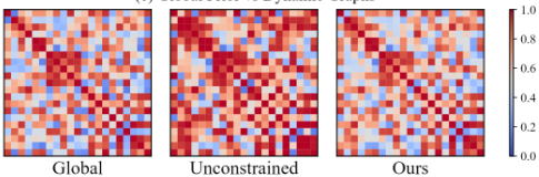
While these methods have achieved some success, in many cases, the dependencies between variables are time-varying and noisy [Huang et al., 2023; Zhao et al., 2023; Liu et al., 2025]. The relationships between variables can change with changes in the overall state or sudden events, and spurious correlations often appear within the time window [Chen et al., 2024a; Lin et al., 2025]. This leads to a dilemma between stability and adaptability (Fig. 1). Using a single global static dependency structure [Wu et al., 2020] can capture general relationships between variables, but it cannot capture the dynamic evolution of these relationships over time. Conversely, if dynamic graph learning is relied upon entirely for flexibility, the model is prone to overfitting to local windows, introducing noise. Especially when the local window is finite, noise can easily be mistaken for the true structure and further amplified during subsequent propagation [Chen et al., 2024b; Hu et al., 2025; Li et al., 2023]. Therefore, this dilemma indicates that we need a new modeling approach: one that can adapt to changes over time and effectively resist noise interference, that is, one that can dynamically change while maintaining structural controllability.
Based on the above discussion, we propose the Constraint-Guided Dynamic Graph Network (ConDyGNet). ConDyGNet first extracts a globally shared basis bank from global correlations, thereby learning common inter-channel interaction patterns. Then, for each time window, the model only needs to predict window-specific mixing weights and combine them with the shared basis to obtain the dependency structure for that time window. We call this global basis, dynamic weights. This approach allows us to restrict the structure to a controlled subspace. ConDyGNet can both learn temporal changes and avoid relearning the structure in each temporal window, maintaining global structural consistency and thus improving model stability. Furthermore, to suppress spurious associations during graph fusion, we decouple "whether a connection exists" from "how strong a connection is": we first obtain sparse edge support through structureaware filtering, and then compute specific weights only on these edges to prevent noise propagation. Our contributions can be summarized as follows:
- We analyze the core issue of inter-channel modeling in MTSF: the trade-off between stability and adaptivity. Static structures cannot capture changes in relationships over time, while unconstrained dynamic graphs are easily disturbed by local spurious correlations.
- We propose ConDyGNet, which follows the principle of global basis, dynamic weights, and decouples structural support from interaction strength. We also introduce a structure-aware filtering mechanism to effectively suppress spurious dependencies before graph fusion.
- Extensive experiments show that ConDyGNet achieves superior performance on multiple public MTSF benchmarks, achieving state-of-the-art results. Ablation studies and stability analysis further validate the benefits of global basis guidance for noise suppression.
2 RelatedWork
2.1 Time Series Forecasting
In recent years, deep learning has played an important role in the development of Multivariate Time Series Forecasting (MTSF). RNN-based methods [Lin et al., 2023] use hidden states to capture past information, but they often face the vanishing gradient problem on long sequences. CNN-based methods [Wu et al., 2023; Luo and Wang, 2024] use convolutional kernels to extract local features. Although they can expand the receptive field to capture longer correlations, they still struggle to model global information because of locality. Transformer-based methods [Zhang and Yan, 2023; Nie et al., 2023; Liu et al., 2024; Wang et al., 2024] use attention mechanisms to capture long-term dependencies, and they have become a mainstream paradigm. However, they may ignore the temporal characteristics of time series, and often require high computational cost for long sequences. MLP-based methods [Zeng et al., 2023; Das et al., 2023] use a simple structure for efficient modeling. Despite these advances, many models ignore inter-channel relationships or fail to model their structure and dynamics. As a result, models cannot effectively handle complex relationships between channels, and may amplify noise-induced spurious correlations during propagation, which reduces prediction accuracy.
2.2 GNNs for Inter-channel RelationModeling
In recent years, graph neural networks (GNNs) have emerged as a crucial paradigm in multivariate time series forecasting (MTSF), primarily due to their ability to explicitly model inter-channel relationships. Early research focused on specific domain tasks such as traffic prediction [Yu et al., 2017; Li et al., 2018; Wu et al., 2019; Cini et al., 2023], where natural spatial connectivity facilitates the direct definition of graph structures. More recent work has applied GNNs to more general MTSF scenarios. Since these scenarios often lack inherent spatial structures, models need to learn latent inter-channel relationships. MTGNN [Wu et al., 2020] can discover latent directed relationship matrices and perform predictions through mix-hop propagation. FourierGNN [Yi et al., 2023] utilizes the frequency domain for message passing, improving the efficiency of capturing long-term dependencies. MSGNet [Cai et al., 2024] enhances model robustness through multi-scale graph propagation. TimeFilter [Hu et al., 2025] filters out irrelevant spatio-temporal edges to achieve fine-grained spatio-temporal modeling. Despite these advancements, existing methods often struggle to effectively suppress noise-induced spurious correlations while capturing dynamically evolving relationships over time. This problem is further exacerbated when the number of channels is large. Therefore, constructing an inter-channel relationship model in MTSF that simultaneously possesses dynamic adaptability and noise resistance remains a challenging task.
3 Preliminaries
For multivariate time series forecasting, we denote X ∈ RC×L as the input time series, where C represents the number of channels and L represents the look-back horizon. Our goal is to forecast the next T time steps Y ∈ RC×T .
To model dynamic inter-channel relationships, we divide X into P patches. We construct a corresponding relationship matrix Ap ∈ RC×C for each patch p. Ap[i, j] represents the gated interaction strength from channel j to channel i in the p-th patch. In our design, Ap is generated jointly by the gate and intensity, and restricted by basis structure constraints. By filtering out suspicious noise edges, our design improves the robustness of the model.
4 Method
4.1 Overview
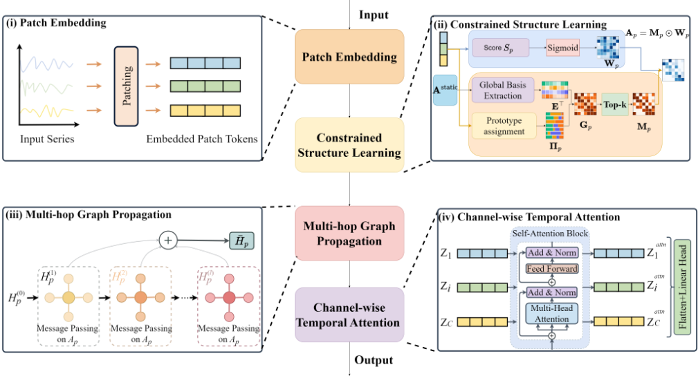
As shown in Fig. 2, the core of ConDyGNet is in the combination of global basis and patch-wise dynamic weights, forming a topology gate for the intensity matrix, which is realized through four key components: (i) Patch Embedding Module divides the input sequence into non-overlapping patches and encodes each patch as a channel token representation H; (ii) Constrained Structure Learning Module constructs a low-rank basis and patch-wise dynamic weights and then filters them to obtain a topology gate, where the dynamic intensity works together with the gate to form a dynamic graph that can effectively suppress noise; (iii) Multi-hop Graph Propagation performs multi-hop message passing on the dynamic graph at the patch level, aggregating neighborhood information to model the relationships between channels; (iv) Channel-wise Temporal Attention uses self-attention at the patch dimension for each channel to capture long-term temporal relationships, and then flattens the sequence and applies a linear projection to generate the outputs.
4.2 Patch Embedding
Inspired by PatchTST [Nie et al., 2023], in this stage, each channel of the input sequence X ∈ RC×L is first divided into non-overlapping patches, and each patch is then mapped to an embedded patch token. Since the process is identical for each channel, we use X to represent the multivariate input and later operate on all channels in parallel. Formally, this process can be formulated as follows:
The length of each patch is S and the number of patches is P = ⌈L/S⌉. The Embedding(·) operation transforms each patch from its original length S to a hidden dimension D through a trainable linear layer, resulting in embedded patch tokens H ∈ RC×P×D .
4.3 Constrained Structure Learning
To inhibit the negative effects of noisy patch-wise dependencies in inter-channel graph construction, we design a constrained structure learning method. The model learns a sparse topology gate from the global basis and uses it to gate patchspecific interaction intensities, thereby yielding a structureconstrained patch-wise dynamic graph Ap ∈ [0, 1]C×C for message passing.
Dynamic Interaction Intensity
We first compute a channel-wise interaction score matrix for each patch. Specifically, we use a standard scaled dot-product scoring mechanism (including learnable projection matrices)
to calculate pairwise interaction scores, and then use a Sigmoid function to map the scores to a bounded range, thus obtaining the intensity matrix. Let Hp = H[:, p, :] ∈ RC×D denote the channel representations of the p-th patch. We compute the pairwise interaction score matrix as
where WQ,WK ∈ RD×D are learnable projection matrices shared across patches. We then obtain the intensity matrix by
where σ(·) denotes the Sigmoid function. We choose Sigmoid instead of Softmax to allow the connection strength of each edge to vary independently, without the constraint of probability normalization.
However, due to the limited patch length, directly computing the intensity matrix is likely to be affected by local noise. Therefore, we introduce a sparse topology gate to further filter out unreliable edges, as detailed below.
Low-Dimensional Basis Construction
To obtain a robust topology gate, we avoid learning an unconstrained patch-specific topology in the full RC×C space, as its O(C 2 ) degrees of freedom per patch can be unstable and prone to overfitting. Inspired by AGCRN [Bai et al., 2020], we construct a set of shared basis modes, reducing the effective complexity to O(CR) with R ≪ C, where R is the rank (i.e., the number of basis modes). Specifically, we maintain a basis bank E ∈ RC×R shared across patches and generate patch-adaptive structure via context-dependent basis mixing, balancing global consistency and local adaptivity.
We initialize E from the training split in an offline manner and only allow a lightweight in-subspace adaptation during training. To obtain a stable spectral anchor, we construct a global residual-affinity matrix Astatic on the training split; its eigendecomposition provides a dominant spectral subspace that captures recurring long-term dependency patterns and constrains the basis bank to mitigate noisy patch-wise drift. Since correlations on raw observations can be dominated by shared trends and external factors, we first remove slow trends to emphasize residual co-movements:
We then compute a scale-invariant residual affinity by cosine similarity and keep non-negative evidence:
where ∥Xs ∥2 ∈ RC denotes the vector of row-wise ℓ2 norms of Xs , and the division is performed element-wise.
Finally, we extract a dominant structural subspace from Astatic by eigendecomposition:
where U is orthonormal and Λ = diag(λ1, . . . , λC), sorted in descending order. Since Astatic summarizes the global residual affinity patterns, its leading eigenvectors capture significant and recurring interaction patterns shared among channels. We only need a few leading eigenvectors, because they preserve most of the structural energy while filtering out noise. Accordingly, we take the top-R eigenvectors as our initial basis E0 = U:,1:R. We then define the learnable basis bank as the product of the initial basis and a learnable transformation matrix:
where Q ∈ RR×R is learnable and initialized as identity. This design aims to add constraints to the basis bank, restricting it to the dominant subspace and preventing it from drifting uncontrollably within the huge solution space. At the same time, the model can still flexibly reweight and rotate the feature patterns according to the specific task through the transformation matrix. Through this strategy of limiting degrees of freedom, the learning process of the topological structure becomes more stable, thus exhibiting stronger robustness when dealing with noisy short-window data.
Context-Aware Basis Mixing
For each patch p, we first calculate the routing weights over the shared basis modes, and then mix them with the basis bank to obtain row-wise structural evidence. Specifically, for channel i in patch p, we obtain a routing representation ψ(Hp(i, :)) and measure its squared Euclidean distance to the mode prototypes {µr}Rr=1 . Here, ψ(·) is a lightweight projection and µr ∈ RD are shared mode prototypes in the routing space, learned end-to-end. We use a softmin-style normalization to convert these distances into mixture coefficients:
The distance-driven routing mechanism ensures that channels with similar patch contexts are mapped to neighboring locations in the routing space, so their mixture weights will be similar. This leads to smooth and interpretable mode assignments. Meanwhile, Gp(i, :) is a weighted mixture over the shared basis bank, which restricts each row to an Rdimensional subspace. It still allows the model to adapt across patches and can naturally form asymmetric directed structures across channels.
Row-wise Topology Gate
We sparsify the structure matrix obtained above by row-wise normalization and Top-k filtration. First, we select only nonnegative entries, and then normalize each row by its offdiagonal maximum:
If maxm̸=i ¯Gp(i,m) = 0, we set all off-diagonal entries in that row to 0. We then keep the strongest off-diagonal candidates per row while always retaining the self-loop:
Here, Top-k(·) selects up to ⌈k(C-1)⌉ largest non-zero entries, where k ∈ (0, 1) is a ratio controlling the sparsity of each row. Top-k is only used for gating: gradients pass through retained entries, while pruned ones receive zero gradients. This ensures that each node can be connected to at most ⌈k(C-1)⌉ off-diagonal edges, and the diagonal entries are fixed to 1.
Finally, we use element-wise fusion to obtain the dynamic graph. The topology gate Mp determines the connectivity andWp provides the interaction intensities:
Here, Ap ∈ [0, 1]C×C denotes the patch-specific weighted propagation graph for message passing.
4.4 Multi-hop Graph Propagation
After obtaining the patch-wise propagation graphs, we perform multi-hop graph propagation [Abu-El-Haija et al., 2019] on each patch to obtain graph-enhanced patch tokens.
Let H(0) p ∈ RC×D denote the channel tokens of patch p. We perform graph propagation with a residual connection to the root state. The propagation is defined as:
where ℓ denotes the propagation depth and β ∈ (0, 1) controls the proportion of the root state retained at each propagation layer. Ap is used directly as the propagation operator for neighborhood aggregation.
We then combine representations from different propagation depths to obtain graph-enhanced patch tokens using fixed and normalized fusion weights:
where {αℓ} are fixed normalized weights. We set {αℓ} using a simple non-increasing decay over hop depth, with αℓ ∝ 1/(ℓ+1), which favors shallow hops. Finally, we stack { ¯Hp}Pp=1 along the patch dimension to form Z ∈ RC×P×D .
4.5 Channel-wise Temporal Attention
To model the inter-patch dependencies for each channel, we use a self-attention block on its patch sequence for each channel independently. Let Zi ∈ RP×D denote the patch sequence of channel i. We use a standard Transformer structure:
Here, LN(·) represents Layer Normalization, Attention(·) is multi-head self-attention and FFN(·) is the positionwise feed-forward network. We collect {Zattn i }Ci=1 to form Zattn ∈ RC×P×D . Finally, Zattn ∈ RC×P×D is flattened and projected to the final output Y ∈ RC×T .
5 Experiments
5.1 Setup
Datasets. We extensively benchmark our method on 8wellestablished datasets, including Weather, Traffic, Electricity, Solar, and four ETT datasets (ETTh1, ETTh2, ETTm1, and ETTm2) [Zhou et al., 2021]. These datasets have been widely used in time series forecasting literature. They cover diverse sampling frequencies and variable dimensions, enabling a fair and rigorous comparison with baseline methods.
Baselines. We compare our method with SOTA representativemethods, includingGNN-basedmethods: TimeFilter [Hu et al., 2025], MSGNet [Cai et al., 2024]; Transformer-based methods: TimeXer [Wang et al., 2024], iTransformer [Liu et al., 2024], PatchTST [Nie et al., 2023]; MLP-based methods: DUET [Qiu et al., 2025], SOFTS [Han et al., 2024], DLinear [Zeng et al., 2023]; CNN-based method: TimesNet [Wu et al., 2023].
Implementation Details. All experiments were implemented using PyTorch and were run on an NVIDIA A800 80GB PCIe GPU. ConDyGNet used the Adam optimizer. To improve training stability, we adopt a hybrid MAE loss which incorporates both the time and frequency domains. For fair comparison, all models used an input length of L=96 and a prediction length of T ∈ {96, 192, 336, 720}, with MSE and MAE used as evaluation metrics. Dataset splitting: The ETT dataset used the official standard 12/4/4-month train/validation/test split; other datasets were split in a 7:1:2 ratio. Models were trained for 10 epochs (30 for Traffic) with an early stopping strategy (patience= 3). The learning rate ranges from {1e-3, 5e-4, 1e-4}, the batch size ranges from {16, 32}, and the dropout ranges from {0.1, 0.3, 0.5}. The patch length ranges from {2, 4, 8, 16, 32, 48}. The number of attention heads is fixed at 4. For the number of basis modes R, 3 is chosen for the ETT dataset, 6 for the Weather dataset, and 16 for all other datasets. The sparsity ratio is set to 0.3, the propagation depth is set to 2, the root-state residual weight is set to β=0.2, and the random seed is fixed at 2021.
5.2 Results
We report the long-term forecasting results in Table 1. Across 8 datasets and 4 forecasting horizons, ConDyGNet achieves the best or tied-best MAE in 30 settings and the best or tiedbest MSE in 25 settings. Remarkably, in 25 out of 32 cases, our method achieves state-of-the-art performance on both metrics simultaneously, demonstrating comprehensive superiority over diverse baselines including Transformers, MLPs, and GNNs.
As shown in Table 1, ConDyGNet consistently achieves the best performance. Notably, the large-scale datasets present substantial challenges due to their high dimensionality and intricate temporal dependencies. ConDyGNet balances stability and adaptivity in modeling time-varying interchannel dependencies through constrained structure learning, yielding consistently strong forecasting accuracy. Quantitatively, on Electricity, ConDyGNet reduces the average MSE/MAE by 9.1%/8.5%, 9.9%/4.5%, and 2.3%/3.5% compared with TimeXer [Wang et al., 2024], DUET [Qiu et al., 2025], and TimeFilter [Hu et al., 2025], respectively.
| Datasets | Ours | TimeFilter | DUET | TimeXer | SOFTS | iTransformer | MSGNet PatchTST | TimesNet | DLinear | ||||
|---|---|---|---|---|---|---|---|---|---|---|---|---|---|
| MAE | MSE | MAE MSE | MAE | MSE MAE | MSE | MAE | MSE MAE | MSE MAE | MSE MAE | MSE MAE | |||
| ETTh1 | MSE MAE MSE 96 0.364 0.388 192 0.412 0.420 336 0.452 0.443 720 0.463 0.456 | 0.370 0.394 0.413 0.420 0.450 0.440 0.448 0.457 | 0.377 0.429 0.471 0.496 | 0.393 0.425 0.446 0.480 | 0.382 0.429 0.468 0.469 | 0.403 0.435 0.448 0.461 | 0.381 0.399 0.435 0.431 0.480 0.452 0.499 0.488 | 0.386 0.441 0.487 0.494 | 0.405 0.390 0.436 0.442 0.458 0.480 0.488 0.494 | 0.411 0.414 0.442 0.460 0.468 0.501 0.488 0.500 | 0.419 0.384 0.445 0.436 0.466 0.491 0.488 | 0.402 0.429 0.469 0.500 0.519 | 0.386 0.400 0.437 0.432 0.481 0.459 0.516 |
| ETTh2 | 96 0.277 0.327 192 0.356 0.378 336 0.403 0.416 720 0.418 | 0.283 0.337 0.362 0.392 0.404 0.424 0.434 0.407 0.433 | 0.296 0.368 0.411 0.412 | 0.345 0.389 0.422 0.434 | 0.286 0.338 0.363 0.389 0.414 0.423 0.408 0.432 | 0.297 0.373 0.410 0.411 | 0.347 0.394 0.426 0.433 | 0.297 0.380 0.428 0.427 | 0.349 0.328 0.400 0.402 0.432 0.435 0.445 0.417 | 0.371 0.302 0.414 0.388 0.443 0.426 0.441 0.431 | 0.348 0.340 0.400 0.402 0.433 0.452 0.446 0.462 | 0.521 0.374 0.414 0.452 0.468 | 0.333 0.387 0.477 0.476 0.594 0.541 0.831 0.657 |
| ETTm1 | 96 0.310 0.347 192 0.353 0.372 336 0.376 0.392 720 0.435 | 0.313 0.354 0.356 0.380 0.386 0.402 0.428 0.452 0.437 | 0.324 0.369 0.404 0.463 | 0.354 0.379 0.402 0.437 | 0.318 0.356 0.362 0.383 0.395 0.407 0.452 0.441 | 0.325 0.375 0.405 0.466 | 0.361 0.389 0.412 0.447 | 0.334 0.377 0.426 0.491 | 0.368 0.391 0.420 0.459 | 0.319 0.366 0.329 0.376 0.397 0.367 0.417 0.422 0.399 0.481 0.458 0.454 | 0.362 0.338 0.385 0.374 0.410 0.410 0.439 0.478 | 0.375 0.387 0.411 0.450 0.474 | 0.345 0.372 0.380 0.389 0.413 0.413 0.453 |
| ETTm2 | 96 0.167 0.249 192 0.231 0.292 336 0.292 0.332 720 0.390 | 0.169 0.255 0.235 0.299 0.293 0.336 0.389 0.390 0.393 | 0.174 0.243 0.304 0.399 | 0.255 0.302 0.341 0.397 | 0.171 0.256 0.237 0.299 0.296 0.338 0.392 0.394 | 0.180 0.246 0.319 0.405 | 0.261 0.306 0.352 0.401 | 0.180 0.250 0.311 0.412 | 0.264 0.309 0.348 0.407 | 0.177 0.262 0.175 0.247 0.307 0.241 0.312 0.346 0.305 0.414 0.403 0.402 | 0.259 0.187 0.302 0.249 0.343 0.321 0.400 0.408 | 0.267 0.309 0.351 0.403 0.554 | 0.193 0.292 0.284 0.362 0.369 0.427 0.522 |
| Weather | 96 0.148 0.186 192 0.197 0.235 336 0.254 0.277 720 0.337 0.332 | 0.153 0.199 0.202 0.246 0.260 0.289 0.342 0.341 | 0.163 0.218 0.274 0.349 | 0.202 0.252 0.294 0.343 | 0.157 0.205 0.204 0.247 0.261 0.290 0.340 0.341 | 0.166 0.217 0.282 0.356 | 0.208 0.253 0.300 0.351 | 0.174 0.221 0.278 0.358 | 0.214 0.254 0.296 0.349 | 0.163 0.212 0.177 0.212 0.254 0.225 0.272 0.299 0.278 0.350 0.348 0.354 | 0.218 0.172 0.259 0.219 0.297 0.280 0.348 0.365 | 0.220 0.196 0.261 0.237 0.306 0.283 0.359 0.345 | 0.255 0.296 0.335 0.381 |
| Electricity | 96 0.129 0.222 192 0.148 0.238 336 0.160 0.252 720 0.182 0.275 | 0.133 0.230 0.154 0.248 0.162 0.261 0.184 0.284 | 0.145 0.163 0.175 0.204 | 0.233 0.248 0.262 0.291 | 0.140 0.242 0.157 0.256 0.176 0.275 0.211 0.306 | 0.143 0.158 0.178 0.218 | 0.233 0.248 0.269 0.305 | 0.148 0.162 0.178 0.225 | 0.240 0.253 0.269 0.317 | 0.165 0.274 0.195 0.184 0.292 0.199 0.195 0.302 0.215 0.231 0.332 | 0.285 0.168 0.289 0.184 0.305 0.198 0.256 0.337 0.220 | 0.272 0.289 0.300 0.320 0.245 | 0.197 0.282 0.196 0.285 0.209 0.301 0.333 |
| Solar | 96 0.185 0.203 192 0.217 0.224 336 0.231 0.238 720 0.239 0.245 | 0.193 0.223 0.226 0.249 0.235 0.261 0.239 0.268 | 0.200 0.228 0.262 0.258 | 0.207 0.233 0.244 0.249 | 0.215 0.295 0.236 0.301 0.252 0.307 0.244 0.305 | 0.200 0.229 0.243 0.245 | 0.230 0.253 0.269 0.272 | 0.203 0.233 0.248 0.249 | 0.237 0.261 0.273 0.275 | 0.208 0.243 0.234 0.258 0.281 0.267 0.293 0.311 0.290 0.290 0.315 0.289 | 0.286 0.250 0.310 0.296 0.315 0.319 0.317 0.338 | 0.292 0.318 0.330 0.337 0.356 | 0.290 0.378 0.320 0.398 0.353 0.415 0.413 |
| Traffic | 96 0.381 0.239 192 0.400 0.249 336 0.419 0.260 720 0.455 0.286 | 0.375 0.251 0.395 0.262 0.414 0.271 0.445 0.289 | 0.407 0.431 0.456 0.509 | 0.252 0.262 0.269 0.292 | 0.428 0.271 0.448 0.282 0.473 0.289 0.516 0.307 | 0.376 0.398 0.415 0.447 | 0.251 0.261 0.269 0.287 | 0.395 0.417 0.433 0.467 | 0.268 0.276 0.283 0.302 | 0.605 0.344 0.544 0.613 0.359 0.540 0.642 0.376 0.551 0.702 0.401 0.586 | 0.359 0.593 0.354 0.617 0.358 0.629 0.375 0.640 | 0.321 0.336 0.336 0.350 0.645 | 0.650 0.396 0.598 0.370 0.605 0.373 0.394 |
5.3 Ablation Analysis
We conducted ablation testing to verify the effectiveness of the ConDyGNet design. We chose four ablation methods and evaluated them on three datasets. The specific implementations are as follows:
- w/o-Constraint: We removed the constrained structure modules and used unconstrained and learned correlation matrices to replace them.
- w/o-Dynamic: We removed dynamics and replaced them with only a global static graph.
- w/o-Intensity: We removed interaction intensity modeling and retained only topology gating.
- w/o-Gate: We removed the topology gate, did not utilize structure filtering, and only used interaction intensity.
Results Analysis. Table 2 shows the results of the ablation study. From the table, we can see that removing any module decreases performance, showing that the design of each module is effective and reasonable. We have summarized the following improvements:
- Improvement of constrained structure: The result of replacing the constrained structure with an unconstrained and learned, patch-specific graph leads to worse performance. This suggests that restricting structure estimation to a controlled basis is very important.
- Improvement of dynamics: After removing dynamics and replacing them with a global static graph, the performance of the model has decreased a lot, especially on Solar. This is because Solar has a higher dimension and more complex inter-channel relationships, making it difficult for a global static graph to adapt to changes over different time periods.
- Improvement of intensity and gate: Examining the results of w/o-Intensity and w/o-Gate variants, we can see that decoupling intensity and gate is essential for robust inter-channel relationships. Filtering out unreliable edges and using intensity on the remaining edges can effectively reduce noise.
| Dataset | Solar | Weather | ETTm1 | |||
|---|---|---|---|---|---|---|
| Metric | MSE | MAE | MSE | MAE | MSE | MAE |
| ConDyGNet | 0.231 | 0.238 | 0.254 | 0.277 | 0.376 | 0.392 |
| w/o-Constraint | 0.235 | 0.240 | 0.257 | 0.281 | 0.385 | 0.399 |
| w/o-Dynamic | 0.259 | 0.254 | 0.257 | 0.279 | 0.379 | 0.394 |
| w/o-Intensity | 0.237 | 0.242 | 0.256 | 0.279 | 0.379 | 0.393 |
| w/o-Gate | 0.236 | 0.240 | 0.257 | 0.280 | 0.381 | 0.396 |
5.4 Model Analysis
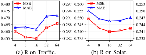
Impact of the Rank R. In the constrained structure learning module, the rank R represents the number of basis modes used for relationship modeling. In principle, R should preserve the main inter-channel interaction patterns while avoiding overfitting to noise, making an appropriate choice of R crucial. We conduct experiments on two representative datasets, Traffic and Solar, with R ∈ {4, 8, 16, 32, 64} under the long-horizon setting with input length L=96 and prediction length T=720. As shown in Fig. 3, the performance on both datasets exhibits a clear U-shaped trend, and the model achieves the best results when R=16. When R is too small, the basis space becomes overly compact, discarding informative interaction patterns and limiting the expressive power of inter-channel relationship modeling. Conversely, when R is too large, many minor and potentially noisy patterns are introduced into the structural subspace, weakening the constraint effect and increasing computational overhead. Overall, an appropriate rank strikes a better balance between model expressiveness and structural regularization.
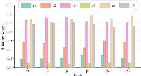
Dynamic Routing Weights. We visualize the dynamic routing weights of each patch on the Weather dataset. For each patch, we compute its routing distribution across R bases and plot the evolution of this distribution along the patch sequence. As shown in Fig. 4, the routing weights exhibit two characteristics. First, most routing weights are concentrated on a few bases, indicating that the inter-channel relationship structure can be well represented with only a small number of bases. Second, the changes in routing weights between adjacent patches are relatively smooth, rather than fluctuating drastically between patches. This suggests that the routing dynamics usually evolve smoothly over time.
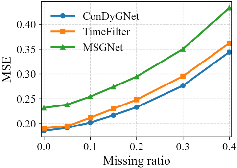
Robustness toMissing-BlockCorruptions. To test the robustness of the models, we conduct missing-block experiments during the testing phase without retraining and observe the changes in MSE for each method as the missing block ratio increases. Fig. 5 shows the results of ConDyGNet and two state-of-the-art GNN-based methods, TimeFilter [Hu et al., 2025] and MSGNet [Cai et al., 2024], on the ECL dataset with an input length of 96, under different missing block ratios ρ ∈ {0, 0.05, 0.10, 0.15, 0.20, 0.30, 0.40}. As ρ increases from 0 to 0.40, the errors of all three methods increase, but ConDyGNet exhibits the slowest degradation and remains consistently lower than TimeFilter and MSGNet. These results indicate that ConDyGNet has stronger robustness to missing-block perturbations. This demonstrates that even with missing values, the global basis can effectively keep the model within a constrained structural subspace, thus significantly improving robustness.
6 Conclusion
Since the relationships between channels in multivariate time series are often time-varying and noisy, we propose ConDyGNet to more robustly capture such dynamic dependencies. ConDyGNet follows the principle of "global basis, dynamic weights": it first decomposes the global relationships into a low-rank basis and calculates mixed weights for each patch to generate a patch-wise propagation graph. Simultaneously, it decouples the topology from the interaction strength through sparse gating, effectively filtering out spurious associations before message passing. Experimental results show that ConDyGNet achieves SOTA performance on eight real-world datasets, demonstrating superior prediction accuracy.
Acknowledgments
This work is supported by the Fundamental and Interdisciplinary Disciplines Breakthrough Plan of the Ministry of Education of China (JYB2025XDXM907).
@inproceedings{ijcai2026p505,
  title     = {ConDyGNet: Constraint-Guided Dynamic Graph Networks for Multivariate Time Series Forecasting},
  author    = {Li, Zhenzhou and Li, Xiang and Niu, Zhibin},
  booktitle = {Proceedings of the Thirty-Fifth International Joint Conference on
               Artificial Intelligence, {IJCAI-26}},
  publisher = {International Joint Conferences on Artificial Intelligence Organization},
  editor    = {Diego Calvanese},
  pages     = {4536--4544},
  year      = {2026},
  month     = {8},
  note      = {Main Track},
  doi       = {10.24963/ijcai.2026/505},
  url       = {https://doi.org/10.24963/ijcai.2026/505},
}
TY - CPAPER TI - ConDyGNet: Constraint-Guided Dynamic Graph Networks for Multivariate Time Series Forecasting AU - Li, Zhenzhou AU - Li, Xiang AU - Niu, Zhibin T2 - Proceedings of the Thirty-Fifth International Joint Conference on Artificial Intelligence, IJCAI-26 PB - International Joint Conferences on Artificial Intelligence Organization PY - 2026 SP - 4536 EP - 4544 DO - 10.24963/ijcai.2026/505 UR - https://doi.org/10.24963/ijcai.2026/505 ER -Copied
Machine-readable versions of this paper, for tools and AI agents:





