
INSHAPE: Instance-Level Shapelets for Interpretable Time-Series Classification
Proceedings of the Thirty-Fifth International Joint Conference on Artificial Intelligence. Main Track. Pages 4456-4464.
https://doi.org/10.24963/ijcai.2026/496
© 2026 International Joint Conferences on Artificial Intelligence
Keywords
- Machine Learning: Feature extraction, selection and dimensionality reduction
- Machine Learning: Classification
- Machine Learning: Time series and data streams
- Machine Learning: Explainable/Interpretable machine learning
Abstract
Discovering shapelets -- i.e., discriminative temporal patterns within time series -- has been widely studied to address the inherent complexity of time-series classification (TSC) and to make model decision-making processes more transparent.
However, existing methods primarily focus on population-level shapelets optimized across the entire dataset, which leads to two fundamental limitations: (i) population-level patterns often misalign with instance-specific features, resulting in suboptimal performance and potentially misleading interpretations, and (ii) most methods treat shapelets as independent entities, overlooking important temporal dependencies and interactions among multiple patterns.
To address these limitations, we propose INSHAPE, an interpretable TSC framework that discovers variable-length, discriminative temporal patterns specific to each time series.
INSHAPE identifies these patterns as non-overlapping segments and models their temporal dependencies, thereby providing clear instance-level interpretations while achieving strong predictive performance.
Furthermore, INSHAPE bridges local and global interpretability through a bottom-up approach, aggregating instance-level shapelets into prototypical (population-level) shapelets.
Extensive experiments on 128 UCR and 30 UEA benchmark datasets show that INSHAPE consistently outperforms state-of-the-art shapelet-based methods while providing more intuitive and interpretable insights.
- [Bagnall et al., 2018] Anthony Bagnall, Hoang Anh Dau, Ja- son Lines, Michael Flynn, James Large, Aaron Bostrom, Paul Southam, and Eamonn Keogh. The uea multivari- ate time series classification archive, 2018. arXiv preprint arXiv:1811.00075, 2018.
- [Bengio et al., 2013] Yoshua Bengio, Nicholas Léonard, and Aaron Courville. Estimating or propagating gradients through stochastic neurons for conditional computation. arXiv preprint arXiv:1308.3432, 2013.
- [Dau et al., 2019] Hoang Anh Dau, Anthony Bagnall, Kaveh Kamgar, Chin-Chia Michael Yeh, Yan Zhu, Shaghayegh Gharghabi, Chotirat Ann Ratanamahatana, and Eamonn Keogh. The ucr time series archive. IEEE/CAA Journal of Automatica Sinica, 6(6):1293-1305, 2019.
- [Dierckx, 1982] Paul Dierckx. A fast algorithm for smooth- ing data on a rectangular grid while using spline functions. SIAM Journal on Numerical Analysis, 19(6):1286-1304, 1982.
- [Grabocka et al., 2014] Josif Grabocka, Nicolas Schilling, Martin Wistuba, and Lars Schmidt-Thieme. Learning time- series shapelets. In Proceedings of the 20th ACM SIGKDD international conference on Knowledge discovery and data mining, pages 392-401, 2014.
- [Grabocka et al., 2015] Josif Grabocka, Martin Wistuba, and Lars Schmidt-Thieme. Scalable discovery of time-series shapelets. arXiv preprint arXiv:1503.03238, 2015.
- [Gumbsch et al., 2020] Thomas Gumbsch, Christian Bock, Michael Moor, Bastian Rieck, and Karsten Borgwardt. En- hancing statistical power in temporal biomarker discovery through representative shapelet mining. Bioinformatics, 36(Supplement 2):i840-i848, 2020.
- [Hills et al., 2014] Jon Hills, Jason Lines, Edgaras Baranauskas, James Mapp, and Anthony Bagnall. Classification of time series by shapelet transformation. Data mining and knowledge discovery, 28(4):851-881, 2014.
- [Hyland et al., 2020] Stephanie L Hyland, Martin Faltys, Matthias Hüser, Xinrui Lyu, Thomas Gumbsch, Cristóbal Esteban, Christian Bock, Max Horn, Michael Moor, Bas- tian Rieck, et al. Early prediction of circulatory failure in the intensive care unit using machine learning. Nature medicine, 26(3):364-373, 2020.
- [Ismail Fawaz et al., 2020] Hassan Ismail Fawaz, Benjamin Lucas, Germain Forestier, Charlotte Pelletier, Daniel F Schmidt, Jonathan Weber, Geoffrey I Webb, Lhassane Idoumghar, Pierre-Alain Muller, and Franc ¸ois Petitjean. Inceptiontime: Finding alexnet for time series classification. Data Mining and Knowledge Discovery, 34(6):1936-1962, 2020.
- [Jang et al., 2016] Eric Jang, Shixiang Gu, and Ben Poole. Categorical reparameterization with gumbel-softmax. arXiv preprint arXiv:1611.01144, 2016.
- [Kacprzyk et al., 2024] Krzysztof Kacprzyk, Tennison Liu, and Mihaela van der Schaar. Towards transparent time series forecasting. In The Twelfth International Conference on Learning Representations, 2024.
- [Killick et al., 2012] Rebecca Killick, Paul Fearnhead, and Idris A Eckley. Optimal detection of changepoints with a linear computational cost. Journal of the American Statisti- cal Association, 107(500):1590-1598, 2012.
- [Kim et al., 2024] Chohee Kim, Mihaela Van Der Schaar, and Changhee Lee. Discovering features with synergistic in- teractions in multiple views. In Forty-first International Conference on Machine Learning, 2024.
- [Lee et al., 2022] Changhee Lee, Fergus Imrie, and Mihaela van der Schaar. Self-supervision enhanced feature selec- tion with correlated gates. In International conference on learning representations, 2022.
- [Li and Zhao, 2023] Yingxiang Li and Xuejing Zhao. Patient- specific warning of epileptic seizure upon shapelets features. Heliyon, 9(11), 2023.
- [Li et al., 2021] Guozhong Li, Byron Choi, Jianliang Xu, Sourav S Bhowmick, Kwok-Pan Chun, and Grace Lai- Hung Wong. Shapenet: A shapelet-neural network ap- proach for multivariate time series classification. In Pro- ceedings of the AAAI conference on artificial intelligence, volume 35, pages 8375-8383, 2021.
- [Lin et al., 2007] Jessica Lin, Eamonn Keogh, Li Wei, and Stefano Lonardi. Experiencing sax: a novel symbolic rep- resentation of time series. Data Mining and knowledge discovery, 15(2):107-144, 2007.
- [Lines et al., 2012] Jason Lines, Luke M Davis, Jon Hills, and Anthony Bagnall. A shapelet transform for time series classification. In Proceedings of the 18th ACM SIGKDD international conference on Knowledge discovery and data mining, pages 289-297, 2012.
- [Liu et al., 2023] Liyuan Liu, Chengyu Dong, Xiaodong Liu, Bin Yu, and Jianfeng Gao. Bridging discrete and backprop- agation: Straight-through and beyond. Advances in Neural Information Processing Systems, 36:12291-12311, 2023.
- [Liu et al., 2025] Zhen Liu, Yicheng Luo, Boyuan Li, Emadeldeen Eldele, Min Wu, and Qianli Ma. Learning soft sparse shapes for efficient time-series classification. International Conference on Machine Learning, 2025.
- [Luo and Wang, 2024] Donghao Luo and Xue Wang. Mod- erntcn: A modern pure convolution structure for general time series analysis. In The twelfth international conference on learning representations, pages 1-43, 2024.
- [Maddison et al., 2016] Chris J Maddison, Andriy Mnih, and Yee Whye Teh. The concrete distribution: A continuous relaxation of discrete random variables. arXiv preprint arXiv:1611.00712, 2016.
- [Mohammadi Foumani et al., 2024] Navid Moham- madi Foumani, Lynn Miller, Chang Wei Tan, Geoffrey I Webb, Germain Forestier, and Mahsa Salehi. Deep learning for time series classification and extrinsic regression: A current survey. ACM Computing Surveys, 56(9):1-45, 2024.
- [Neves et al., 2021] Inês Neves, Duarte Folgado, Sara Santos, Marília Barandas, Andrea Campagner, Luca Ronzio, Fed- erico Cabitza, and Hugo Gamboa. Interpretable heartbeat classification using local model-agnostic explanations on ecgs. Computers in biology and medicine, 133:104393, 2021.
- [Qin et al., 2025] Xuewei Qin, Yi Sun, Jiemin Ji, and Jun Li. Fetalet: interpretable fetal heart rate anomaly detection via shapelet learning. Complex & Intelligent Systems, 11(11):1- 16, 2025.
- [Qu et al., 2024] Eric Qu, Yansen Wang, Xufang Luo, Wen- qiang He, Kan Ren, and Dongsheng Li. Cnn kernels can be the best shapelets. In The Twelfth International Conference on Learning Representations, 2024.
- [Rakthanmanon and Keogh, 2013] Thanawin Rakthanmanon and Eamonn Keogh. Fast shapelets: A scalable algorithm for discovering time series shapelets. In proceedings of the 2013 SIAM International Conference on Data Mining, pages 668-676. SIAM, 2013.
- [Salvador and Chan, 2007] Stan Salvador and Philip Chan. Toward accurate dynamic time warping in linear time and space. Intelligent data analysis, 11(5):561-580, 2007.
- [Vaswani et al., 2017] Ashish Vaswani, Noam Shazeer, Niki Parmar, Jakob Uszkoreit, Llion Jones, Aidan N Gomez, Łukasz Kaiser, and Illia Polosukhin. Attention is all you need. Advances in neural information processing systems, 30, 2017.
- [Wen et al., 2025] Yunshi Wen, Tengfei Ma, Ronny Luss, De- barun Bhattacharjya, Achille Fokoue, and Anak Agung Julius. Shedding light on time series classification using interpretability gated networks. In The Thirteenth Interna- tional Conference on Learning Representations, 2025.
- [Williams, 1992] Ronald J Williams. Simple statistical gradient-following algorithms for connectionist reinforce- ment learning. Machine learning, 8(3):229-256, 1992.
- [Wu et al., 2022] Haixu Wu, Tengge Hu, Yong Liu, Hang Zhou, Jianmin Wang, and Mingsheng Long. Timesnet: Temporal 2d-variation modeling for general time series analysis. International Conference on Learning Represen- tations, 2022.
- [Ye and Keogh, 2009] Lexiang Ye and Eamonn Keogh. Time series shapelets: a new primitive for data mining. In Pro- ceedings of the 15th ACM SIGKDD international confer- ence on Knowledge discovery and data mining, pages 947- 956, 2009.
- [Yoon et al., 2018] Jinsung Yoon, James Jordon, and Mihaela Van der Schaar. Invase: Instance-wise variable selection using neural networks. In International conference on learning representations, 2018.
- [Zuo et al., 2023] Rundong Zuo, Guozhong Li, Byron Choi, Sourav S Bhowmick, Daphne Ngar-yin Mah, and Grace LH Wong. Svp-t: A shape-level variable-position transformer for multivariate time series classification. In Proceedings of the AAAI Conference on Artificial Intelligence, volume 37, pages 11497-11505, 2023.
References were extracted automatically from the PDF and may contain errors.
Full text extracted automatically from the PDF; figures, tables and equations may differ. The PDF is the version of record.
1 Introduction
Shapelets are highly informative subsequences that distinguish between classes in time-series data [Ye and Keogh, 2009]. By discovering class-discriminative temporal patterns across an entire population, shapelets provide global interpretability, revealing which temporal features differentiate one class from another. In addition, shapelets also support local interpretability by pinpointing whether and where these patterns occur within individual instances - typically through posthoc overlay. These two levels of interpretability are particularly valuable in high-stakes domains such as healthcare [Hyland et al., 2020; Gumbsch et al., 2020; Li and Zhao, 2023; Qin et al., 2025; Neves et al., 2021]: global explanations help clinicians identify population-level temporal biomarkers, while local explanations provide case-specific insights for understanding individual-level diagnoses.
1 An extended version of this paper with supplementary material is available at https://arxiv.org/abs/2605.20088.
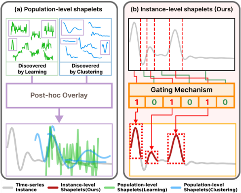
While recent deep learning models for time-series classification (TSC) achieve strong predictive performance, their inherent complexity has driven the development of shapelet-based methods that integrate interpretable temporal patterns directly into the prediction process [Li et al., 2021; Zuo et al., 2023; Qu et al., 2024; Wen et al., 2025; Liu et al., 2025]. However, these methods face two critical limitations when applied to instance-level prediction and interpretation. First, most methods rely on population-level shapelets optimized to capture broad class characteristics, which often result in patterns that are overly smoothed or poorly aligned with individual instances. Second, despite the dependence of TSC decisions on the interaction, order, or relative position of multiple temporal patterns [Mohammadi Foumani et al., 2024], existing methods typically discover shapelets independently, and therefore fail to capture these crucial temporal dependencies. Figure 1(a) illustrates the consequence of these limitations: when overlapped and input-misaligned population-level shapelets are presented as local explanations, they obscure which temporal patterns are truly discriminative for a specific instance, thereby limiting the reliability of instance-level interpretation.
Motivated by the above limitations, we propose INSHAPE (INstance-level SHAPElets) 2 , a novel interpretable-by-design framework for TSC. Instead of relying on a fixed set of globally optimized shapelets, INSHAPE discovers discriminative temporal patterns directly from each input time series while capturing their temporal dependencies. Specifically, INSHAPE first partitions each time series into variable-length, statistically coherent time-series segments. It then employs a gating mechanism - comprising an amortized selector and a temporal predictor - to identify segments that are most predictive of the target label. This enables the discovery of instance-level shapelets that account for complex temporal interactions, providing local explanations that faithfully reflect the input's temporal structure as shown in Figure 1(b). Extensive experiments on 128 UCR and 30 UEA benchmark datasets demonstrate that INSHAPE achieves superior classification performance compared to state-of-the-art shapeletbased models. Furthermore, INSHAPE offers a novel pathway to global interpretability. By aggregating discovered discriminative instance-level shapelets across the dataset, our framework constructs a set of high-quality, population-level shapelets. When combined with our selector's localization capability, these population-level shapelets reveal not only which global patterns are identified, but also where and how they manifest across instances, bridging the gap between local and global interpretability.
2 RelatedWork
2.1 Population-level Shapelet Discovery
In TSC, shapelets [Ye and Keogh, 2009] are widely used to provide global interpretability by identifying temporal patterns that frequently occur in specific classes. Early shapelet discovery methods relied on exhaustive search to evaluate all possible candidate subsequences, which is computationally prohibitive for large datasets. To address this, more recent works have focused on improving efficiency by pruning candidates with symbolic aggregate approximation [Lin et al., 2007; Rakthanmanon and Keogh, 2013], clustering candidate patterns [Grabocka et al., 2015; Zuo et al., 2023; Li et al., 2021], and learning shapelets directly as learnable parameters via gradient descent [Grabocka et al., 2014; Qu et al., 2024; Wen et al., 2025]. Despite these advances, existing methods treat candidate segments independently during the discovery process. Hence, by ignoring the temporal dependencies among segments, these methods are restricted to interpreting individual patterns in isolation, failing to capture how the collective interaction and ordering of multiple patterns jointly contribute to the final classification.
2 Code: https://github.com/nshuhsn/INSHAPE IJCAI.
2.2 Population-level Shapelets for Classification
Shapelet transform-based methods [Hills et al., 2014; Lines et al., 2012] leverage population-level shapelets for instancelevel prediction and interpretation by representing each time series as a vector of minimum distances from a fixed set of shapelets. The resulting distance-based representation of each time series is then utilized by various types of classifiers, including linear models [Grabocka et al., 2014; Wen et al., 2025], SVMs [Li et al., 2021], and neural networks [Qu et al., 2024; Zuo et al., 2023], which learn class-discriminative decision boundaries based on the relative similarity. Local interpretability is typically provided through post-hoc analysis by overlaying each shapelet at its closest matching location within a given time-series instance. However, such post-hoc overlays often fail to capture instance-specific discriminative patterns, leading to local explanations that are weakly aligned with the true temporal patterns of individual time series. Moreover, because the shapelet transform primarily encodes the presence of shapelets via distance-based representations, positional information and temporal dependencies among multiple shapelets are often discarded [Mohammadi Foumani et al., 2024] (See Supplementary A). While recent work attempts to mitigate this limitation by incorporating population-level shapelets into deep neural networks that model temporal dependencies for TSC [Zuo et al., 2023], these dependencies are still not considered during the shapelet discovery stage.
Unlike prior works, INSHAPE selects discriminative segments at the instance level while accounting for their temporal dependencies to predict the target class during the selection process. The most closely related work is SoftShape [Liu et al., 2025], which partitions time-series segments into top-k "important" and "unimportant" groups, encoding them separately and modeling their interactions to construct the final prediction. However, because unimportant segments - which do not correspond to any shapelet patterns - still contribute to the prediction, it remains unclear which specific temporal patterns are truly responsible for the TSC. In contrast, INSHAPE employs hard gating via Bernoulli sampling [Maddison et al., 2016; Yoon et al., 2018; Kim et al., 2024; Lee et al., 2022]. This stochastic selection process learns to flexibly select any number of important time-series segments while ensuring the classification depends exclusively on the selected segments for each time-series instance. Consequently, INSHAPE captures complex temporal interactions among instance-level shapelets whose contributions are directly attributable, thereby enabling clearer and more reliable local interpretations.
3 ProblemFormulation
Consider a dataset comprising n time-series instances, i.e., D = {(x(i) 1:T , y(i) )}ni=1 where x1:T = (x1, . . . , xT ) ∈ RT denotes a univariate time series of length T and y ∈ {1, . . . , C} is its associated label in a C-class classification task. For notational simplicity, we focus on the univariate setting; however, our formulation naturally extends to p-dimensional multivariate time series x(i) 1:T ∈ Rp×T . We will omit the dependency for the instance index (i) when it is clear from the context.
Definition 3.1 (Partial Segmentation). Given a time-series instance x1:T , a valid partial segmentation divides it into M non-overlapping segments, each potentially of varying length, as described below:
where each segment sm = (xτ sm , . . . , xτ em ) with τ sm ≤ τ em < τ sm+1 for all m ∈ {1, . . . ,M - 1}. The number of segments M can range from 1 to T , i.e., 1 ≤ M ≤ T .
A time series is considered fully segmented if τ sm+1 = τ em + 1 for all m ∈ {1, . . . ,M - 1}, and we denote such a segmentation as ¯s(x1:T ) = (¯ s1, . . . , ¯ sM). Unlike full segmentation, partial segmentation selects only a subset of the time series, such that the total number of selected time points may be less than T , i.e., ∑Mm=1 |sm| ≤ T . This reflects our focus on identifying only the most informative regions rather than covering the entire sequence. Each time-series instance can have multiple valid partial segmentations that vary not only in the number of segments but also in their individual lengths. Denote S(x1:T ) be the set of all such valid partial segmentations of x1:T . Then, we can formally define instance-level shapelets as follows:
Definition 3.2 (Instance-level Shapelets). The instance-level shapelet of a time series x1:T is defined as the most discriminative partial segmentation with respect to the target label:
subject to the constraints ∑M∗ m=1 |s∗m| ≤ δ1 and |s∗m| ≥ δ2 for m ∈ {1, . . . ,M ∗ }, where δ1 limits the total length of selected segments and δ2 constrains a minimum segment length. These constraints ensure that the selected segments remain concise and provide compact interpretations.
Challenges. Unfortunately, solving the optimization problem in (2) is highly non-trivial for several reasons. First, it requires estimating the objective function - specifically, the conditional distribution of the target label given any arbitrary partial segmentation. Second, the space of possible partial segmentations for each instance, i.e., S(x1:T ), is combinatorially large, making the discrete optimization computationally intractable. Third, the solution must satisfy interpretability constraints such that selecting a small number of segments while ensuring each segment is sufficiently long to capture semantically meaningful patterns.
4 INSHAPE: INstance-level SHAPElet
To overcome the challenges outlined above, we reformulate instance-level shapelet discovery as a problem of selecting discriminative segments from a fully segmented time series. To do so, we introduce a gating mechanism designed to distinguish between discriminative and non-discriminative segments. Given a fully-segmented time series, ¯s(x1:T ), we define a binary gate vector as follows:
where each gate gm is a binary vector of length τ em - τ sm + 1, set to all ones if the corresponding segment is selected, and all zeros otherwise. The instance-level shapelets of x1:T can then be discovered by optimizing the gate vector to maximize the following objective:
where ⊙ denotes element-wise multiplication. The resulting instance-level shapelet is thus given by s∗ = ¯s(x1:T ) ⊙ g∗ .
Solving this optimization problem in (4) presents two key challenges: (Time Series Segmentation) We must fully segment each time-series instance into meaningful temporal patterns. This is crucial to avoid the computationally intractable burden of discrete optimization across all possible full segmentations. (Amortized Gate Vector Optimization) To manage the cost of solving a per-instance optimization problem, we amortize this expense across a population of input time series. This is achieved by training a neural network to learn inputdependent gate vectors for segment selection. We will describe each in turn in the following subsections.
4.1 Segmenting Time Series intoMeaningful Patterns
To reduce the combinatorial burden of exploring all possible full segmentations of a time-series instance, we instead focus on identifying meaningful transition points that delineate segment boundaries. Motivated by recent studies [Kacprzyk et al., 2024] that break down time series into interpretable patterns, we propose the following two properties that such transition points should satisfy for a desirable full segmentation:
- Transition points should be frequent in regions exhibiting abrupt and large fluctuations, as these often correspond to extreme values informative for predicting the target class y.
- Transition points should be sparse in regions showing gradual, smooth variations, as such segments typically represent coherent trends relevant to y.
Hence, we adopt two representative transition point algorithms that reflect these properties from different perspectives:
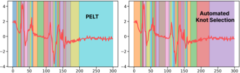
Automated Knot Selection [Dierckx, 1982]: Denote T = {τ1, . . . , τK} be a set of knots (i.e., transition points) that partition [0, T] into K - 1 intervals, with B-spline basis functions km(t) used on each interval [τm, τm+1] for m ∈ {1, . . . ,K - 1}. To automatically determine the placement and number of these knots, we employ an iterative method that begins with a single segment (i.e., K = 2). In each step, a new knot is inserted into the interval with the largest residual until the following inequality holds:
where c1(·, ·) is the residual (e.g., squared error) and β > 0 is the smoothing parameter.
PELT Algorithm [Killick et al., 2012]: The Pruned Exact Linear Time (PELT) algorithm identifies transition points by minimizing a penalized sum of segment-wise costs using dynamic programming with pruning:
where T = {τ1 . . . τK} is the set of transition points. The term c2(·) represents the cost associated with each segment (e.g., using an RBF-based cost function), and β > 0 penalizes the number of change points |T | to prevent over-segmentation.
Consequently, these transition point algorithms identify statistically coherent segments, ¯s(x1:T ), thereby avoiding the computational burden of full segmentation and providing segments with meaningful temporal patterns that serve as a basis for intuitive, reliable explanations (Figure 2). In this work, we adopt PELT as our default segmentation algorithm due to its computational efficiency; the effect of utilizing B-spline and uniform segmentation is also provided in Section 5.3.
4.2 Amortized Gate Vector Optimization
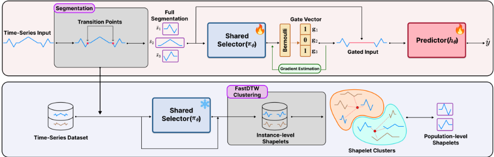
The optimization in (4) is inherently memoryless, requiring independent computation for each input time series without leveraging patterns from previously seen (and possibly similar) instances. To overcome this inefficiency, we reformulate the problem using amortized optimization by introducing a gating mechanism. Specifically, we define a selector (parameterized by ϕ) that stochastically maps a varying length time-series segment ¯ sm to a single binary gate gm. To achieve the gate vector g, each segment is processed by the shared selector using a masked self-attention mechanism that captures the representation of its shape as illustrated in Figure 3. Formally, the selector, πϕ : Rτ em-τ sm+1 → [0, 1], outputs a Bernoulli parameter based on ¯ sm, such that gm ∼ Bern(πϕ(¯ sm)). We also define a predictor hθ : RT → [0, 1]C that estimates the conditional distribution over class labels given any selected subset of segments. This leads to the following joint optimization:
where λ > 0 is a coefficient that balances the selected number of segments. The element-wise product ¯s(x1:T ) ⊙ g masks non-selected segments with redundant zero-terms rather than removing them, thereby preserving the original temporal context and positional information for the predictor. Additionally, since the discrete sampling of g makes (7) non-differentiable with respect to ϕ, we adopt ReinMax [Liu et al., 2023], a second-order accurate gradient estimator for binary random variables that reduces gradient bias compared to StraightThrough Estimators (STE) [Bengio et al., 2013]. Notably, other gradient estimation techniques such as STGS [Jang et al., 2016], REINFORCE [Williams, 1992] can also be applied within our framework.
We implement the selector, πϕ, using Transformer [Vaswani et al., 2017] followed by an MLP layer, with both components shared across all segments to efficiently process variablelength segments in a single forward pass. For the predictor, hθ, we utilize an InceptionTime architecture [Ismail Fawaz et al., 2020], whose multi-level convolutional filters are adept at capturing diverse dependencies among the selected segments; we further evaluate alternative predictor architectures in Section 5.3. Through joint optimization, the InceptionTime predictor generates rich and informative gradient signals that are propagated back to the selector. This feedback loop is crucial: it enables the selector to implicitly learn and account for inter-segment dependencies, even though the selector processes each segment individually.
Once trained, INSHAPE provides local interpretability for an individual time-series instance by first applying the segmentation algorithm and then leveraging the selector's output; the segments corresponding to the activated gates are identified as instance-level shapelets.
4.3 Bridging Local and Global Interpretability
Local interpretability alone is not sufficient to answer population-level questions, such as identifying which temporal patterns are commonly important for distinguishing between classes across the dataset. To address this, we adopt a selectthen-cluster strategy to derive population-level shapelets. Specifically, we first use the trained selector to extract instancelevel shapelets from all time-series instances. These selected segments are then clustered via FastDTW [Salvador and Chan, 2007], which naturally handles varying-length time-series segments, and the resulting cluster centroids are defined as the population-level shapelets (see Figure 3). By restricting the candidate pool to selected discriminative segments rather than clustering raw subsequences, INSHAPE substantially reduces the search space and enables the discovery of more representative and meaningful population-level shapelets.
Building on the discovered population-level shapelets, our framework goes beyond identifying global patterns by explicitly bridging local and global interpretations and providing quantitative insights into their class-wise correspondences:
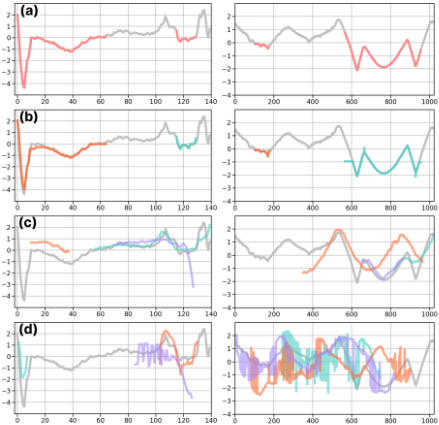
- Bridging Local and Global Interpretations: Each instance-level shapelet is assigned to its nearest populationlevel shapelet based on the FastDTW distance. This assignment connects global trends to local explanations by revealing where the discovered population-level shapelets manifest within individual instances (see Figure 4(b)).
- Quantitative Global Insights: We compute the class-wise frequency of each population-level shapelet assigned to timeseries instances. This reveals which global patterns commonly characterize each class. Visualizing these frequent patterns across the population provides insights into shared temporal structures and dependencies (see Figure 5).
Detailed procedures for population-level shapelet discovery, local interpretation using population-level shapelets, and the computation of quantitative global insights are provided in Supplementary Material Section B.4.
| LTS | ShapeNet | ShapeConv | SVP-T | SBM | Ours | |
|---|---|---|---|---|---|---|
| IS | ✗ | ✗ | ✗ | ✗ | ✗ | ✓ |
| PS | ✓ | ✓ | ✓ | ✓ | ✓ | ✓ |
| SDw/ TD | ✗ | ✗ | ✗ | ✗ | ✗ | ✓ |
| Pred w/ TD | ✗ | ✗ | ✗ | ✓ | ✗ | ✓ |
5 Experiments
We evaluate INSHAPE on the UCR archive (128 univariate datasets) [Dau et al., 2019] and the UEA archive (30 multivariate datasets) [Bagnall et al., 2018], comparing against six representative shapelet-based methods summarized in Table 1. All experiments follow established evaluation protocols from prior works [Liu et al., 2025; Wen et al., 2025].
- In Section 5.1, we compare classification accuracy and interpretability against baselines, showing that INSHAPE achieves superior performance with clearer interpretations.
- In Section 5.2, we show how population-level shapelets can be used for local and global interpretation.
- In Section 5.3, we conduct ablation studies to analyze the effects of segmentation strategies and predictor architectures. Implementation details, baseline configurations, and metric definitions are provided in Supplementary Material Section B.
5.1 Classification Performance and Interpretability
Performance Analysis. Table 2(a) summarizes the average classification accuracy and ranking statistics on the UCR and UEA datasets. For a fair comparison, we use the interpretable variant of SoftShape; details of this modification and comparison with the original model are provided in Supplementary Material Section B. Across all baselines, INSHAPE achieves the highest average accuracy and the best overall ranking. This highlights that preserving instance-specific information and modeling temporal dependencies are crucial for accurate TSC. Local Interpretability Analysis. For local interpretation, existing shapelet-based methods typically overlay discovered shapelets on the input time series at positions with the smallest distance. We compare local interpretability between INSHAPE and three representative shapelet transform-based baseline methods on the UCR and UEA datasets in Table 2(b). To quantify this, we measure the following metrics for the top-k most important shapelets (ranked by absolute linear classifier weights) and the complete set of all available shapelets:
- Coverage: Proportion of the input time series covered by
| Univariate (UCR 128) | |||||||
|---|---|---|---|---|---|---|---|
| Metric | LTS | Shape Net | SVP-T | Shape Conv | SBM | Soft Shape | Ours |
| Avg. Acc ↑ | 0.6262 | 0.7213 | 0.7018 | 0.7479 | 0.7375 | 0.7820 | 0.8405 |
| Avg. Rank ↓ | 5.797 | 4.371 | 4.277 | 4.117 | 3.938 | 3.105 | 2.395 |
| Wins/Draws | 116 | 93 | 102 | 108 | 98 | 82 | - |
| Losses | 12 | 35 | 26 | 20 | 30 | 46 | - |
| Top-1 | 2 | 30 | 16 | 9 | 29 | 0 | 46 |
| Top-3 | 11 | 46 | 48 | 50 | 49 | 84 | 105 |
Multivariate (UEA 30)
| Metric | LTS | Shape Net | SVP-T | Shape Conv | SBM | Ours |
|---|---|---|---|---|---|---|
| Avg. Acc ↑ | 0.7150 | 0.6306 | 0.6783 | 0.6655 | 0.7277 | 0.7429 |
| Avg. Rank ↓ | 3.183 | 4.950 | 3.700 | 4.050 | 2.567 | 2.550 |
| Wins/Draws | 16 | 24 | 25 | 22 | 16 | - |
| Losses | 14 | 6 | 5 | 8 | 14 | - |
| Top-1 | 3 | 3 | 3 | 5 | 10 | 11 |
| Top-3 | 19 | 6 | 13 | 10 | 22 | 23 |
| Baseline Methods (UCR 128) | Baseline Methods (UEA 30) | ||||||
|---|---|---|---|---|---|---|---|
| Metric (Avg.) | LTS | Shape Net | SBM | Metric (Avg.) | LTS | Shape Net | SBM |
| Coverage (Top-1) | 0.3950 | 0.2840 | 0.4478 | Coverage (Top-1) | 0.4379 | 0.2953 | 0.4943 |
| Coverage (Top-2) | 0.5564 | 0.4554 | 0.5872 | Coverage (Top-2) | 0.5813 | 0.4546 | 0.6487 |
| Coverage (Top-3) | 0.6493 | 0.5827 | 0.6806 | Coverage (Top-3) | 0.6769 | 0.5469 | 0.7290 |
| Coverage (Full) | 0.9852 | 0.8935 | 0.9814 | Coverage (Full) | 0.9845 | 0.7289 | 0.9797 |
| Overlap (Top-1) | 0.0000 | 0.0000 | 0.0000 | Overlap (Top-1) | 0.0000 | 0.0000 | 0.0000 |
| Overlap (Top-2) | 0.2734 | 0.1310 | 0.3033 | Overlap (Top-2) | 0.2910 | 0.1301 | 0.3490 |
| Overlap (Top-3) | 0.4160 | 0.2581 | 0.4398 | Overlap (Top-3) | 0.4236 | 0.2432 | 0.4934 |
| Overlap (Full) | 0.9727 | 0.7685 | 0.9679 | Overlap (Full) | 0.9714 | 0.5760 | 0.9653 |
| Acc (Top-1) | 0.4163 | 0.3246 | 0.4016 | Acc (Top-1) | 0.2345 | 0.3072 | 0.2516 |
| Acc (Top-2) | 0.4089 | 0.3439 | 0.4147 | Acc (Top-2) | 0.2496 | 0.2868 | 0.2784 |
| Acc (Top-3) | 0.4025 | 0.3438 | 0.4217 | Acc (Top-3) | 0.2497 | 0.3253 | 0.2921 |
| Acc (Full) | 0.6262 | 0.7213 | 0.7375 | Acc (Full) | 0.7150 | 0.6306 | 0.7277 |
| Ours (UCR 128) | Ours (UEA 30) | ||||||
| Avg. Shapelet Num | 2.4151 | Avg. Shapelet Num | 1.5266 | ||||
| Avg. Coverage | 0.4949 | Avg. Coverage | 0.5539 | ||||
| Avg. Overlap | 0.0000 | Avg. Overlap | 0.0000 | ||||
| Avg. Acc | 0.8405 | Avg. Acc | 0.7429 | ||||
| LTS | Shape Net | SVP-T | Shape Conv | SBM | Soft Shape | Ours (Pop.) | |
|---|---|---|---|---|---|---|---|
| Avg. Acc ↑ | 0.6542 | 0.7601 | 0.7233 | 0.7876 | 0.772 | 0.7863 | 0.8145 |
| Avg. Rank ↓ | 5.944 | 3.889 | 4.278 | 3.444 | 3.778 | 3.500 | 3.167 |
Table 3: Classification performance using population-level shapelets in place of instance-level shapelets on 18 UCR datasets.
shapelets. Lower coverage indicates more compact explanations that focus on the most critical temporal regions.
- Overlap: Proportion of temporal overlap among selected shapelets. Lower overlap provides clearer interpretations by avoiding redundant highlighting of the same regions.
- Shapelet Num: Average number of instance-level shapelets selected per instance.
In multivariate settings, Coverage and Overlap are measured separately for each channel and then averaged across channels.
In Table 2(b), INSHAPE selects an average of 2.4 and 1.5 instance-level shapelets per time series on the UCR and UEA datasets, respectively. We therefore compare INSHAPE against baselines using their top-1, top-2 and top-3 shapelets. Under these sparse settings, INSHAPE achieves comparable coverage to baselines while exhibiting zero overlap by architectural design, clearly identifying distinct discriminative regions per instance. In contrast, baselines show substantial overlap (13-44% on UCR, 0-35% on UEA) even across the most important shapelets, obscuring which patterns drive predictions. Restricting baseline methods to make predictions solely on the top-k shapelets leads to a substantial drop in classification accuracy, as evidenced by the top-1 and top-2 results. To recover the original performance, these methods need to utilize the entire shapelet set. This results in near-complete coverage (>98%) and overlap (>96%) for a given time-series instance, demonstrating that a sparse, focused local interpretation is not achievable with these methods. In contrast, INSHAPE achieves superior prediction performance while relying exclusively on a small set of non-overlapping temporal regions for each time series, thereby providing clearer and more intuitive local interpretations. Figure 4 shows this distinction: baseline methods produce overlapping, misaligned explanations, while INSHAPE provides compact, non-overlapping segments that offer clearer explanations. Similar trends are observed in the UEA datasets (see Supplementary Material Section C.1).
5.2 Instance-level to Population-level Shapelets
In this subsection, we evaluate the population-level shapelets derived by INSHAPE. We derive population-level shapelets, denoted as P = {p1, . . . , pnP }, by clustering the discriminative instance-level shapelets extracted from all training timeseries instances as described in Section 4.3 (see Supplementary Material Algorithm 1 for details).
Faithfulness of Population-level Shapelets. To validate that population-level shapelets preserve instance-level discriminative information, we replace each instance-level shapelet with its nearest population-level counterpart (based on FastDTW distance), mask all non-selected regions, and then evaluate classification performance. As shown in Table 3, INSHAPE with population-level shapelets achieves the highest average accuracy (0.8145) and the best average rank (3.167), confirming that our bottom-up approach produces faithful populationlevel shapelets.
Quantitative Global Insights. To provide global insights, we compute the usage frequency uc,k for each class c, by counting the number of instance-level shapelets from class-c instances that are assigned to each population-level shapelet pk. The normalized frequency ¯uc,k = uc,k/ ∑k′ uc,k′ quantifies how frequently each class relies on specific population-level shapelets (see Supplementary Material Algorithm 3).
Figure 5 illustrates this global interpretation on the ECG5000 dataset. We first select the top-3 most frequently used shapelets for each class and take their union, resulting in 5 representative shapelets: {p0, p1, p5, p8, p12}. Figure 5(a) presents the class-wise usage proportions ¯uc,k. Although these population-level shapelets are shared across classes, their usage proportions differ substantially, indicating that class distinctions arise not only from which shapelets appear, but also from their combinations and relative frequencies.
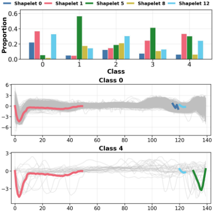
To further investigate these differences, Figure 5(b) and (c) illustrate population-level shapelets overlaid on the timeseries instances with Class 0 and 4, which have a similar shapelet composition but with different proportions. While both classes are characterized by Shapelet 1 (pink) appearing in the early time steps, Class 0 predominantly relies on Shapelet 12 (light blue) in later time steps, whereas Class 4 relies more on Shapelet 5 (green). This comparison underscores that different temporal dependencies among the same set of shapelets serve as a critical discriminative factor between classes. Moreover, the localized regions identified for Class 0 closely align with the instance-level discriminative regions shown in Figure 4, demonstrating consistency between local and global interpretations. Overall, these results show that our framework extends naturally beyond instance-level explanations, enabling rich global insights such as class-wise shapelet utilization and analysis of temporal dependencies.
5.3 Ablation Study
We perform ablation studies on the penalty parameter β in the PELT algorithm, the choice of transition point algorithms, and the predictor architectures, using the 18 UCR datasets following prior work [Liu et al., 2025].
Sensitivity Analysis on the Segmentation Parameter. We use PELT [Killick et al., 2012] as the default transition point algorithm. To ensure consistent segmentation behavior across datasets with varying sequence lengths, we normalize the penalty parameter β in (6) as ¯ β = β/T and tune ¯ β as the hyperparameter. The actual penalty is then computed as β = ¯ β × T . Table 4 summarizes the average ACC, coverage, and the number of discovered shapelets under different ¯ β values. When ¯ β
| ¯ β | Avg. Acc ↑ | Avg. Coverage | Avg. Shapelet Num |
|---|---|---|---|
| 0.01 | 0.8370 | 0.5347 | 2.3371 |
| 0.1∗ | 0.8677 | 0.4834 | 2.7396 |
| 1 | 0.8230 | 0.5591 | 1.7816 |
| 5 | 0.8444 | 0.6979 | 1.1171 |
| 10 | 0.7901 | 0.8170 | 0.9358 |
| Fixed Length | Segmentation | |||
|---|---|---|---|---|
| Metric | W= 1 | W= 2 | B-Spline | PELT |
| Avg. Acc ↑ | 0.7992 | 0.7666 | 0.8288 | 0.8677 |
| Avg. Rank ↓ | 2.6389 | 3.1944 | 2.2222 | 1.9444 |
| Avg. Coverage | 0.5299 | 0.5146 | 0.5019 | 0.4834 |
| Avg. Shapelet Num | 5.4933 | 4.4152 | 2.6570 | 2.7396 |
| TimesNet | ModernTCN | InceptionTime | |
|---|---|---|---|
| Avg. Acc ↑ | 0.7855 | 0.8209 | 0.8651 |
| Avg. Coverage | 0.5569 | 0.5295 | 0.4871 |
| Avg. #S | 2.4431 | 2.3396 | 2.6608 |
is too small, the algorithm produces excessive transition points, leading to over-segmentation that fragments even smooth temporal trends into meaningless patterns. Conversely, when ¯ β is too large, the algorithm becomes overly conservative and misses important transitions. The default (¯ β = 0.1) provides the best trade-off, confirming that the two transition point properties for desirable segmentation described in Section 4.1 are critical for the instance-level shapelet discovery.
Segmentation algorithm comparison. Table 5 compares fixed-length segmentation against adaptive methods (B-Spline and PELT). Adaptive methods outperform fixed-length approaches across all metrics, achieving higher accuracy with fewer shapelets. These results confirm that statistically coherent regions identified by adaptive segmentation align well with discriminative patterns in time series.
Predictor architecture. To demonstrate INSHAPE's robustness across different predictor architectures, we evaluate performance using two recent time-series classification models as the predictor [Luo and Wang, 2024; Wu et al., 2022]. As shown in Table 6, INSHAPE maintains strong performance with both architectures, demonstrating its compatibility with diverse predictors that can capture temporal dependencies to provide informative gradient signals to the selector.
6 Conclusion
We propose INSHAPE, an interpretable-by-design framework for TSC that discovers instance-level shapelets through variable-length segmentation and a gating mechanism, enabling precise alignment with input time series and capturing the underlying temporal dependencies. Furthermore, by adopting a select-then-cluster strategy, INSHAPE derives population-level shapelets that provide better global insight. This unified perspective is particularly valuable for high-stakes domains such as healthcare.
Ethical Statement
While our framework offers both local and global interpretability for TSC through both instance-level and population-level shapelets, the discovered temporal patterns should be validated by domain experts before deployment in high-stakes applications. This is particularly important in healthcare settings, where our method could be used to identify temporal biomarkers or support clinical decision-making. We emphasize that INSHAPE is intended to augment, not replace, expert judgment. In this work, we evaluate our method on publicly available UCR and UEA benchmark datasets, which do not contain personally identifiable information. Any future application to sensitive domains such as clinical diagnostics should follow appropriate ethical guidelines and data governance protocols established by the respective institutions.
Acknowledgements
We thank the reviewers for their comments and suggestions. We also thank Professor Eamonn Keogh and the contributors to the UCR Time Series Classification Archive. This work is supported by the National Research Foundation of Korea (NRF) grant funded by the Korea government (MSIT) (No. RS-202400358602) and the Institute of Information & Communications Technology Planning & Evaluation (IITP) grant funded by the Korea government (MSIT), Artificial Intelligence Graduate School Program (No. RS-2019-II190079, Korea University), the Artificial Intelligence Star Fellowship Support Program to nurture the best talents (No. RS-2025-02304828), and the AI Research Hub Project (No. RS-2024-00457882).
Contribution Statement
Seongjun Lee and Seokhyun Lee contributed equally to this work. Changhee Lee is the corresponding author.
@inproceedings{ijcai2026p496,
  title     = {INSHAPE: Instance-Level Shapelets for Interpretable Time-Series Classification},
  author    = {Lee, Seongjun and Lee, Seokhyun and Lee, Changhee},
  booktitle = {Proceedings of the Thirty-Fifth International Joint Conference on
               Artificial Intelligence, {IJCAI-26}},
  publisher = {International Joint Conferences on Artificial Intelligence Organization},
  editor    = {Diego Calvanese},
  pages     = {4456--4464},
  year      = {2026},
  month     = {8},
  note      = {Main Track},
  doi       = {10.24963/ijcai.2026/496},
  url       = {https://doi.org/10.24963/ijcai.2026/496},
}
TY - CPAPER TI - INSHAPE: Instance-Level Shapelets for Interpretable Time-Series Classification AU - Lee, Seongjun AU - Lee, Seokhyun AU - Lee, Changhee T2 - Proceedings of the Thirty-Fifth International Joint Conference on Artificial Intelligence, IJCAI-26 PB - International Joint Conferences on Artificial Intelligence Organization PY - 2026 SP - 4456 EP - 4464 DO - 10.24963/ijcai.2026/496 UR - https://doi.org/10.24963/ijcai.2026/496 ER -Copied
Machine-readable versions of this paper, for tools and AI agents:





