
Vector-Quantized Discrete Latent Factors Meet Financial Priors: Dynamic Cross-Sectional Stock Ranking Prediction for Portfolio Construction
Proceedings of the Thirty-Fifth International Joint Conference on Artificial Intelligence. Main Track. Pages 4421-4429.
https://doi.org/10.24963/ijcai.2026/492
Keywords
- Multidisciplinary Topics and Applications: Finance
- Machine Learning: Applications
Abstract
Predicting cross-sectional stock returns is challenging due to low signal-to-noise ratios and evolving market regimes. Classical factor models offer interpretability but limited flexibility, while deep learning models achieve strong performance yet often underutilize financial priors. We address this gap with PRISM-VQ (PRior-Informed Stock Model with Vector Quantization), a dynamic factor framework that integrates expert prior factors, vector-quantized discrete latent factors learned from cross-sectional structure, and a structure-conditioned Mixture-of-Experts to generate time-varying factor loadings. Vector quantization acts as an information bottleneck that suppresses noise while capturing robust market structure, with discrete codes serving both as latent factors and as routing signals for temporal expert specialization. Experiments on CSI 300 and S&P 500 show consistent improvements in cross-sectional return prediction and portfolio performance over strong baselines while preserving interpretability. Our code is available at https://github.com/finxlab/PRISM-VQ.
- [Alaygut and Sefer, 2025] Tuna Alaygut and Emre Sefer. Hypergraph neural networks to predict stock movements by exploring higher-order relationships. In Proceedings of the 6th ACM International Conference on AI in Finance, pages 700-708, 2025.
- [Cao et al., 2024] Zhiyuan Cao, Jiayu Xu, Chengqi Dong, Peiwen Yu, and Tian Bai. Matcc: A novel approach for ro- bust stock price prediction incorporating market trends and cross-time correlations. In Proceedings of the 33rd ACM International Conference on Information and Knowledge Management, pages 187-196, 2024.
- [Chen and Guestrin, 2016] Tianqi Chen and Carlos Guestrin. Xgboost: A scalable tree boosting system. In Proceedings of the 22nd acm sigkdd international conference on knowl- edge discovery and data mining, pages 785-794, 2016.
- [Chen et al., 2020] Ting Chen, Simon Kornblith, Moham- mad Norouzi, and Geoffrey Hinton. A simple framework for contrastive learning of visual representations. In In- ternational conference on machine learning, pages 1597- 1607. PmLR, 2020.
- [Chen et al., 2024] Weijun Chen, Shun Li, Xipu Yu, Heyuan Wang, Wei Chen, and Tengjiao Wang. Automatic de- biased temporal-relational modeling for stock investment recommendation. In Proceedings of the Thirty-Third Inter- national Joint Conference on Artificial Intelligence, pages 1999-2008, 2024.
- [Chung et al., 2014] Junyoung Chung, Caglar Gulcehre, KyungHyun Cho, and Yoshua Bengio. Empirical evalua- tion of gated recurrent neural networks on sequence mod- eling. arXiv preprint arXiv:1412.3555, 2014.
- [Cochrane, 2011] John H Cochrane. Presidential address: Discount rates. The Journal of finance, 66(4):1047-1108, 2011.
- [Du et al., 2024] Kelvin Du, Rui Mao, Frank Xing, and Erik Cambria. Explainable stock price movement pre- diction using contrastive learning. In Proceedings of the 33rd ACM International Conference on Information and Knowledge Management, pages 529-537, 2024.
- [Duan et al., 2022] Yitong Duan, Lei Wang, Qizhong Zhang, and Jian Li. Factorvae: A probabilistic dynamic fac- tor model based on variational autoencoder for predicting cross-sectional stock returns. In Proceedings of the AAAI conference on artificial intelligence, volume 36, pages 4468-4476, 2022.
- [Duan et al., 2025] Yitong Duan, Weiran Wang, and Jian Li. Factorgcl: A hypergraph-based factor model with tempo- ral residual contrastive learning for stock returns predic- tion. In Proceedings of the AAAI Conference on Artificial Intelligence, volume 39, pages 173-181, 2025.
- [Fama and French, 1992] Eugene F Fama and Kenneth R French. The cross-section of expected stock returns. the Journal of Finance, 47(2):427-465, 1992.
- [Fama and French, 1993] Eugene F Fama and Kenneth R French. Common risk factors in the returns on stocks and bonds. Journal of financial economics, 33(1):3-56, 1993.
- [Gu et al., 2021] Shihao Gu, Bryan Kelly, and Dacheng Xiu. Autoencoder asset pricing models. Journal of Economet- rics, 222(1):429-450, 2021.
- [Hwang et al., 2023] Yoontae Hwang, Junhyeong Lee, Da- ham Kim, Seunghwan Noh, Joohwan Hong, and Yongjae Lee. Simstock: Representation model for stock similari- ties. In Proceedings of the Fourth ACM International Con- ference on AI in Finance, pages 533-540, 2023.
- [Israel et al., 2020] Ronen Israel, Bryan T Kelly, and To- bias J Moskowitz. Can machines' learn'finance? Journal of Investment Management, 2020.
- [Jensen et al., 2023] Theis Ingerslev Jensen, Bryan Kelly, and Lasse Heje Pedersen. Is there a replication crisis in finance? The Journal of Finance, 78(5):2465-2518, 2023.
- [Kim et al., 2025] Namhyoung Kim, Seung Eun Ock, and Jae Wook Song. Factorvqvae: Discrete latent factor model via vector quantized variational autoencoder. Knowledge- Based Systems, 318:113460, 2025.
- [Lea et al., 2017] Colin Lea, Michael D Flynn, Rene Vidal, Austin Reiter, and Gregory D Hager. Temporal convolu- tional networks for action segmentation and detection. In proceedings of the IEEE Conference on Computer Vision and Pattern Recognition, pages 156-165, 2017.
- [Li et al., 2024] Tong Li, Zhaoyang Liu, Yanyan Shen, Xue Wang, Haokun Chen, and Sen Huang. Master: Market- guided stock transformer for stock price forecasting. In Proceedings of the AAAI Conference on Artificial Intelli- gence, volume 38, pages 162-170, 2024.
- [Loshchilov and Hutter, 2017] Ilya Loshchilov and Frank Hutter. Decoupled weight decay regularization. arXiv preprint arXiv:1711.05101, 2017.
- [Paszke et al., 2019] Adam Paszke, Sam Gross, Francisco Massa, Adam Lerer, James Bradbury, Gregory Chanan, Trevor Killeen, Zeming Lin, Natalia Gimelshein, Luca Antiga, et al. Pytorch: An imperative style, high- performance deep learning library. Advances in neural in- formation processing systems, 32, 2019.
- [Perez et al., 2018] Ethan Perez, Florian Strub, Harm De Vries, Vincent Dumoulin, and Aaron Courville. Film: Visual reasoning with a general conditioning layer. In Pro- ceedings of the AAAI conference on artificial intelligence, volume 32, 2018.
- [Sharpe, 1964] William F Sharpe. Capital asset prices: A theory of market equilibrium under conditions of risk. The journal of finance, 19(3):425-442, 1964.
- [Shazeer et al., 2017] Noam Shazeer, Azalia Mirhoseini, Krzysztof Maziarz, Andy Davis, Quoc Le, Geoffrey Hin- ton, and Jeff Dean. Outrageously large neural net- works: The sparsely-gated mixture-of-experts layer. arXiv preprint arXiv:1701.06538, 2017.
- [Song et al., 2025] Lingyun Song, Haodong Li, Siyu Chen, Xinbiao Gan, Binze Shi, Jie Ma, Yudai Pan, Xiaoqi Wang, and Xuequn Shang. Multi-scale temporal neural network for stock trend prediction enhanced by temporal hyper- edge learning. Proceedings of the IJCAI, Montreal, QC, Canada, pages 16-22, 2025.
- [Su et al., 2024] Jianlin Su, Murtadha Ahmed, Yu Lu, Shengfeng Pan, Wen Bo, and Yunfeng Liu. Roformer: En- hanced transformer with rotary position embedding. Neu- rocomputing, 568:127063, 2024.
- [Van Den Oord et al., 2017] Aaron Van Den Oord, Oriol Vinyals, et al. Neural discrete representation learning. Advances in neural information processing systems, 30, 2017.
- [Vaswani et al., 2017] Ashish Vaswani, Noam Shazeer, Niki Parmar, Jakob Uszkoreit, Llion Jones, Aidan N Gomez, Łukasz Kaiser, and Illia Polosukhin. Attention is all you need. Advances in neural information processing systems, 30, 2017.
- [Xiang et al., 2024] Quanzhou
- Xiang, Zhan Chen, Qi Sun, and Rujun Jiang. Rsap-dfm: Regime-shifting adaptive posterior dynamic factor model for stock returns predic- tion. In Proceedings of the Thirty-Third International Joint Conference on Artificial Intelligence, IJCAI-24. Interna- tional Joint Conferences on Artificial Intelligence Organi- zation, 2024. IJCAI
- [Yang et al., 2020] Xiao Yang, Weiqing Liu, Dong Zhou, Jiang Bian, and Tie-Yan Liu. Qlib: An ai- oriented quantitative investment platform. arXiv preprint arXiv:2009.11189, 2020.
- [Yoo et al., 2021] Jaemin Yoo, Yejun Soun, Yong-chan Park, and U Kang. Accurate multivariate stock movement pre- diction via data-axis transformer with multi-level contexts. In Proceedings of the 27th ACM SIGKDD Conference on Knowledge Discovery & Data Mining, pages 2037-2045, 2021.
- [Zhang and Hua, 2025] Lu Zhang and Lei Hua. Major issues in high-frequency financial data analysis: A survey of so- lutions. Mathematics, 13(3):347, 2025.
- [Zhao et al., 2024] Yilei Zhao, Wentao Zhang, Tingran Yang, Yong Jiang, Fei Huang, and Wei Yang Bryan Lim. Storm: A spatio-temporal factor model based on dual vec- tor quantized variational autoencoders for financial trad- ing. arXiv preprint arXiv:2412.09468, 2024.
References were extracted automatically from the PDF and may contain errors.
Full text extracted automatically from the PDF; figures, tables and equations may differ. The PDF is the version of record.
1 Introduction
Predicting cross-sectional stock returns remains a fundamental challenge at the intersection of finance and machine learning due to persistently low signal-to-noise ratios (SNRs), complex cross-asset dependencies, and frequent regime shifts [Israel et al., 2020; Zhang and Hua, 2025]. Classical linear factor models [Sharpe, 1964; Fama and French, 1992; Fama and French, 1993] provide strong interpretability through economically grounded factors and loadings, but their limited expressiveness restricts their ability to capture nonlinear interactions and time-varying dynamics. This limitation has contributed to the proliferation of the so-called "factor zoo" [Cochrane, 2011], highlighting the difficulty of robust factor discovery.
Recent neural approaches to cross-sectional return prediction largely fall into two categories. Factor-based methods integrate neural networks within factor model structures. Autoencoder-based approaches [Gu et al., 2021; Duan et al., 2022; Kim et al., 2025] learn latent factors via reconstruction objectives, but their reliance on continuous latent representations often provides insufficient regularization under low-SNR conditions and struggles with temporal non-stationarity. In contrast, architecture-centric deep learning methods employ modern sequence models such as Transformers [Yoo et al., 2021; Li et al., 2024; Cao et al., 2024] to model spatio-temporal dependencies directly from data. Despite their expressive power, these models typically lack explicit structural priors, which reduces robustness under distribution shifts and limits interpretability.
∗Corresponding author
Across prior work, three recurring limitations emerge: (1) insufficient regularization of continuous latent representations in noisy environments; (2) structure-agnostic temporal modeling that fails to condition on evolving cross-sectional structure; and (3) underutilization of domain priors, where established financial knowledge is weakly exploited despite its stabilizing potential.
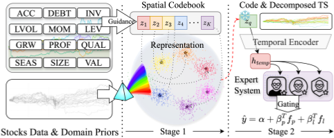
To address these limitations, we propose PRISM-VQ (PRior-Informed Stock Model with Vector Quantization), a unified framework for cross-sectional stock return prediction that integrates discrete representation learning, structureconditioned temporal modeling, and domain-informed priors within a factor-based interpretation (Figure 1). 1 PRISM- VQ consists of three components. First, it learns vectorquantized latent factors through a joint vector quantization and contrastive learning objective [Chen et al., 2020], where the learned codebook [Van Den Oord et al., 2017] acts as an information bottleneck that suppresses noise while preserving cross-sectional structure. Second, it introduces a structure-conditionedMixture-of-Experts (MoE) [Shazeer et al., 2017] built on Transformers, where discrete codes serve as gating signals to generate dynamic factor loadings. Third, it incorporates domain-specific prior factors [Jensen et al., 2023] as stabilizing anchors that maintain interpretability and robustness under distribution shifts.
1 An extended version of this paper, including a technical appendix with additional architectural details, implementation details, robustness analyses, and supplementary experiments, is available at https://arxiv.org/abs/2605.13407.
We summarize our contributions as follows:
- We propose PRISM-VQ, a factor-based framework that combines financial prior factors, vector-quantized discrete latent factors, and structure-conditioned temporal modeling for cross-sectional stock rank prediction.
- We demonstrate that vector quantization provides an effective inductive bias for cross-sectional representation learning, consistently outperforming continuous latent alternatives in noisy financial settings.
- We introduce a discrete-code-gated MoE mechanism that enables structure-conditioned dynamic factor loading generation while preserving a clear factor interpretation and supporting scalable conditional computation.
- We conduct experiments on CSI 300 and S&P 500, where PRISM-VQ achieves the state-of-the-art performance, including RankIC of 0.0646 and 0.0141, and Sharpe ratios of 1.57 and 0.67, respectively.
2 RelatedWorks
2.1 Machine Learning-Based Factor Models
Factor models have long been central to asset pricing, from the CAPM [Sharpe, 1964] to the Fama-French models [Fama and French, 1992]. Although interpretable, their linear structure limits expressiveness in modern markets. Autoencoder asset pricing [Gu et al., 2021] introduced neural networks to learn nonlinear factor structures, followed by extensions such as FactorVAE [Duan et al., 2022] and FactorVQVAE [Kim et al., 2025], which employs vector quantization [Van Den Oord et al., 2017] for discrete latent factors. Later work incorporated additional structure, including graph-based industry modeling [Duan et al., 2025] and regime-aware dynamics [Xiang et al., 2024]. Despite these advances, most methods remain autoencoder-based, limiting temporal modeling capacity and underutilizing financial priors. PRISM-VQ addresses these limitations by combining discrete factor learning with Transformer-based temporal modeling and explicit domain-informed priors.
2.2 Deep Learning for Stock Prediction
Another line of work adopts end-to-end deep learning without explicit factor structures. Transformer-based models have been particularly influential. DTML [Yoo et al., 2021] modeled inter-stock dependencies with attention, MASTER [Li et al., 2024] alternated intra- and inter-stock attention, and MATCC [Cao et al., 2024] incorporated trend decomposition. While effective, these models typically lack interpretable factor representations, weakly encode domain knowledge, and show limited robustness under regime shifts. More recently, explicit relational modeling has been explored through temporal-relational graphs and hypergraph structures [Chen et al., 2024; Song et al., 2025; Alaygut and Sefer, 2025]. These methods rely on predefined or extracted relational topologies, whereas PRISM-VQ learns implicit cross-sectional structure through a discrete codebook without requiring relational preprocessing, enabling transferability across markets. PRISM-VQ retains the expressive power of Transformers while preserving factor interpretability by using them to generate dynamic factor loadings conditioned on learned cross-sectional structure.
2.3 Representation Learning for Finance
The low SNRs of financial data place strong demands on representation learning. Contrastive learning has been explored to learn robust stock embeddings [Du et al., 2024; Hwang et al., 2023]. Vector quantization offers a complementary approach by introducing a discrete information bottleneck that suppresses noise and promotes stable pattern reuse. Recent work has applied vector quantization to identify persistent market structure; for example, STORM [Zhao et al., 2024] employs dual VQ-VAEs to capture spatiotemporal patterns, while FactorVQVAE [Kim et al., 2025] introduces discrete latent factors via a single-stage VQ objective. PRISM-VQ differs from both by combining contrastiveregularized VQ with structure-conditioned MoE routing and explicit financial priors within a unified two-stage framework. To our knowledge, PRISM-VQ is the first framework to integrate vector-quantized discrete factors, contrastive representation learning, expert prior factors, and discrete-codeconditioned temporal modeling within a unified factor-based modeling framework.
3 ProblemFormulation
We study cross-sectional stock return prediction. At each decision time t, the objective is to predict returns for Nt stocks over the next ∆ days for ranking-based portfolio construction. Unless otherwise specified, all quantities are measured at time t, and we omit the explicit time index in symbols such as xi, X, fp, yi, and ˆ yi .
3.1 Data and Factor Model Framework
Each stock i is associated with temporal features xi ∈ RT×C , where T is the lookback window and C is the feature dimension. Stacking all stocks yields the cross-sectional tensor X = {xi}Nt i=1 ∈ RNt×T×C . We also observe P expert prior factors fp ∈ RP , such as value, size, and momentum. The prediction target yi corresponds to the return from t + 1 to t + ∆.
Returns are modeled using a dynamic factor structure:
where αi is the intercept, βp,i and βl,i are loadings on prior and learned factors, fl,i denotes learned latent factors, and
ϵi is idiosyncratic noise. Unlike classical factor models with static linear loadings, both loadings and latent factors are generated by nonlinear mappings:
where Φloading and Φfactor are deep neural networks with parameters θ.
3.2 Modeling Challenges
Cross-sectional stock return prediction faces several challenges: (i) extremely low SNRs, (ii) complex and evolving cross-sectional dependencies, (iii) non-stationary market regimes requiring adaptive factor loadings, and (iv) the need for interpretability consistent with financial theory. PRISMVQ addresses these challenges through a two-stage learning paradigm, where the spatial learning stage discovers discrete latent factors via vector quantization and the temporal learning stage generates dynamic factor loadings using structureconditioned expert networks.
4 ProposedModel
4.1 Overview: Two-Stage Learning
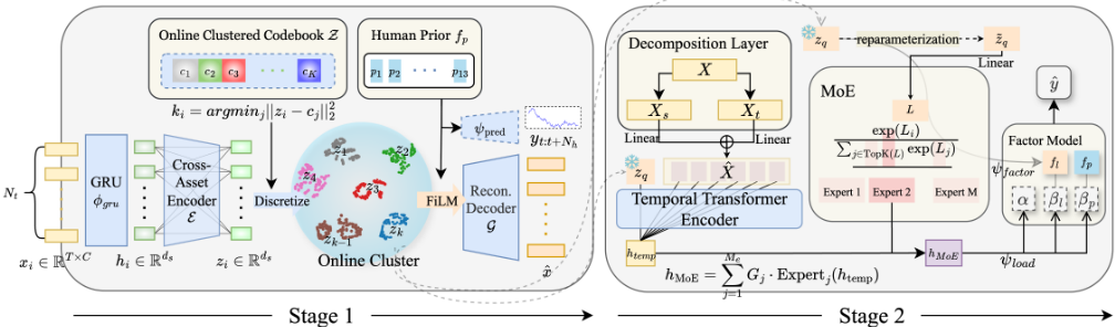
PRISM-VQ decouples cross-sectional structure discovery from time-varying factor loading generation through a twostage framework. Stage 1 (Spatial Learning) learns a discrete codebook and stock-level assignments via vector quantization, mapping codes to latent factor values. Stage 2 (Temporal Learning) generates dynamic factor loadings using a Transformer-based MoE, with expert routing conditioned on the discrete codes. After Stage 1, the codebook is fixed, while stock assignments may vary over time (Figure 2).
Stage 1: Code assignment. At time t, Stage 1 models discrete code assignments conditioned on cross-sectional features and prior factors:
Each discrete code zq,i ∈ Rds is then mapped to a latent factor value
Stage 2: Code-conditioned loading generation. Let βi = (αi, βp,i, βl,i) denote the full set of factor loadings. Conditioned on the discrete code zq,i, Stage 2 generates dynamic loadings via a code-conditioned MoE:
where ej denotes the event of routing to expert j. This conditions temporal modeling on learned cross-sectional structure while preserving a factor interpretation.
4.2 Spatial Learning: Discrete Cross-Sectional Factor Discovery
Cross-Sectional Feature Extraction
Each stock i is associated with features xi ∈ RT×C . We first encode temporal dynamics using a GRU encoder ϕgru:
To capture cross-sectional interactions at time t, we stack all embeddings into H = [h1; . . . ; hNt ] ∈ RNt×ds and apply a cross-asset Transformer encoder E:
Through self-attention, each zi aggregates information from related stocks, forming a representation suitable for discrete clustering.
Vector Quantization for Discrete Factor Learning
We discretize the continuous embeddings using a learnable codebook Z = {ck}Kk=1 ⊂ Rds . Each embedding is assigned to its nearest codeword:
This discretization introduces a finite prototype space that acts as a strong inductive bias under low SNRs. It (i) suppresses idiosyncratic noise by snapping embeddings to recurring cross-sectional prototypes, (ii) limits effective model capacity through a bounded set of codewords, and (iii) encourages sample sharing among stocks assigned to the identical code, yielding stable and interpretable clusters. Since codewords are reused over time, the learned codes naturally separate persistent cross-sectional structures from time-varying factor sensitivities in the two-stage design.
To enable end-to-end training despite the nondifferentiable assignment, we adopt the straight-through estimator [Van Den Oord et al., 2017] and optimize
where sg(·) denotes the stop-gradient operator.
Contrastive Learning for Semantic Clustering
Nearest-neighbor quantization alone may yield arbitrary partitions. We therefore introduce a codebook contrastive objective [Chen et al., 2020]:
where τ is a temperature parameter and sim(u, v) = -∥u - v∥2. This objective contrasts each embedding against all codeword prototypes, explicitly enlarging the margin between the assigned codeword and competing codewords. As a result, clustering is guided by cross-sectional semantics rather than purely geometric proximity.
Reconstruction and Auxiliary Prediction
Pure clustering can produce stable but weakly predictive representations, while pure prediction may fail to extract reusable structure. We therefore introduce two auxiliary tasks to regularize the discrete codes, zq,i.
Reconstruction. A decoder G reconstructs input features from the quantized code, conditioned on prior factors via FiLM (Feature-wise Linear Modulation) [Perez et al., 2018]:
This conditioning encourages the learned codes to remain consistent with the expert prior information.
Multi-horizon prediction. To retain forward-looking signals, we further regularize the codes through multi-horizon return prediction:
Spatial Learning Objective
Then, the following multi-task objective is optimized:
Stage 1 outputs the discrete codes zq,i and the corresponding latent factor values fl,i via Eq.(5), which are subsequently used in Stage 2.
4.3 Temporal Learning: Structure-Conditioned Dynamic Factor Loadings
Temporal Context Encoding with a Structure Token
Given zq,i from Stage 1, we encode temporal context to generate dynamic factor loadings. Let zq,i ∈ Rds and let the temporal encoder operate in Rdt . We optionally decompose each input sequence into trend and residual components and project them to dimension dt:
To inject cross-sectional structure, we prepend zq,i as a structure token (projected to dt if ds ̸= dt) and apply a temporal Transformer encoder T with RoPE (Rotary Position Embedding) [Su et al., 2024]:
Structure-Conditioned MoE for Dynamic Loadings and Return Prediction
Dynamic factor loadings are generated via a structureconditioned MoE, where zq,i determines expert routing.
Stochastic gating mechanism. We compute the expertwise mean and scale parameters from the discrete code:
and sample pre-activations via reparameterization:
We obtain logits Li = ψg(˜ gi) ∈ RMe , select the top-k experts Ki = Topk(Li), and apply a local softmax to define the gating weights:
By construction, ∑j Gi,j = 1 and ∥Gi∥0 = k.
Expert aggregation and loading projection. Each expert ξj : Rdt →Rdt is implemented as a lightweight MLP:
Expert outputs are aggregated and projected to dynamic factor loadings:
Return prediction. We compute the learned factor values from the discrete codes and predict returns:
where αi ∈ R, βp,i ∈ RP , βl,i ∈ Rds , and fp ∈ RP .
Training Objective with Load-Balancing Regularization
The temporal learning stage minimizes the mean squared error with a standard load-balancing regularizer [Shazeer et al., 2017] to prevent expert collapse:
4.4 Two-Stage Training Procedure
Stage 1: Spatial learning. We optimize Lspatial in Eq.(14) to learn the temporal encoder ϕgru, cross-asset encoder E, codebook Z, and auxiliary modules G and ψpred. This stage produces discrete codes zq,i and latent factor values fl,i.
Stage 2: Temporal learning. We fix Z and optimize Ltemporal in Eq.(23) to train the temporal Transformer T , MoE gating and experts, and loading projection ψload, with Stage 1 discrete codes acting as structural conditioning signals for expert routing and factor construction.
Design rationale. The two stages are decoupled to avoid codebook collapse [Van Den Oord et al., 2017] and to enforce an information bottleneck. Stage 1 compresses crosssectional variation into a stable discrete structure, while Stage 2 conditions temporal modeling on this representation without co-adapting the codebook. 2
5 Experiments and Results
We evaluate PRISM-VQ on two major stock markets and conduct a comprehensive empirical study to assess its effectiveness, robustness, and interpretability. All reported results are computed on a strictly out-of-sample test period spanning 2022 to 2024, using identical data preprocessing pipelines and train-validation-test splits across all methods.
Research Questions. Our experiments are designed to address the following questions:
- RQ1 (Overall effectiveness). Does PRISM-VQ improve cross-sectional rank prediction and portfolio performances compared to strong baseline methods?
- RQ2 (Component validity). How do the three core components, namely expert prior factors, the discrete codebook, and the structure-conditionedMoE, individually contribute to overall performance?
- RQ3 (Robustness). How sensitive is PRISM-VQ to key hyperparameters, including codebook size, number of experts, and portfolio top-K selection?
- RQ4 (Interpretability). Do the learned discrete codes capture economically meaningful structure beyond standard factor taxonomies?
- RQ5 (Expert specialization). Do different experts specialize in distinct market conditions while maintaining stable behavior over time?
2 Additional architectural and implementation details can be found in Technical Appendix A of the extended version.
5.1 Experimental Setting
Datasets and Protocol
We evaluate PRISM-VQ on two major stock markets, CSI 300 (China) and S&P 500 (U.S.), using data from Qlib [Yang et al., 2020]. At each trading date t, we use contemporaneous index constituents to avoid survivorship bias. Input features are Alpha158 factors with a lookback window of T = 20 days. The prediction target is the 5-day forward return, yi,t = (priceclose i,t+5 - priceclose i,t+1 )/priceclose i,t+1 , where priceclose i,t+k denotes the close price of stock i k trading days after decision time t. We additionally include 1- to 9day forward returns as auxiliary targets for Lpred. Expert prior factors consist of P=13 factor returns from the JKP Global Factor Library [Jensen et al., 2023], computed using information up to t - 1 and aggregated as 20-day cumulative values. 3
We adopt chronological splits with training from 2009 to 2019, validation from 2020 to 2021, and testing from 2022 to 2024. Features are normalized using RobustZScoreNorm, missing values are forward-filled with Fillna, and training targets are cross-sectionally ranknormalized per date using CSRankNorm.
Baselines
We compare PRISM-VQ against representative baselines from three categories. General machine learning methods include XGBoost [Chen and Guestrin, 2016], GRU [Chung et al., 2014], TCN [Lea et al., 2017], and Transformer [Vaswani et al., 2017]. Factor-based methods include CAE [Gu et al., 2021], VAE [Duan et al., 2022], and VQVAE [Kim et al., 2025]. Architecture-centric deep learning methods include DTML [Yoo et al., 2021], MASTER [Li et al., 2024], and MATCC [Cao et al., 2024]. All baselines use identical data splits and preprocessing pipelines, with hyperparameters tuned on the validation set.
Evaluation Metrics
We evaluate performance using two complementary criteria. First, cross-sectional ranking accuracy is measured by daily RankIC and RankICIR. Second, portfolio performance is evaluated using a TopK-DropN strategy with K=30 and N=5, reporting annualized return (AR), maximum drawdown (MDD), and Sharpe ratio. 4 All portfolio results incorporate transaction costs of 5 basis points at open and 15 basis points at close.
Implementation Details
PRISM-VQ is implemented in PyTorch [Paszke et al., 2019] and trained on a single NVIDIA RTX 3090 GPU. All experiments are repeated with five random seeds. In Stage 1, we use a representation dimension ds=128 with a GRU encoder, a VQ codebook of size K=512, and a cross-asset Transformer with one layer and two attention heads. This stage is trained for up to 50 epochs. In Stage 2, we use a temporal dimension dt=64 and a temporal Transformer with RoPE, using two heads for CSI 300 and four heads for S&P 500, with dropout set to 0.1. The Transformer is followed by an MoE of lightweight MLP experts, with Me=2 (top-1) for CSI 300 and Me=8 (top-4) for S&P 500. Stage 2 is trained for up to 50 epochs with the codebook fixed. Optimization is performed using AdamW [Loshchilov and Hutter, 2017] with a learning rate 10-4 , LambdaLR scheduling, gradient clipping at 1.0, and early stopping with patience 15. We set λcommit=0.25, λcontra=1, λpred=10-4 , and λbalance=10-2 for CSI 300 and 10-3 for S&P 500.
3 Additional details on factor construction and preprocessing are available in Technical Appendix B of the extended version.
4 Formal definitions of the evaluation metrics and additional details of the portfolio construction protocol are available in Technical Appendix C and D of the extended version.
| Market | Model | RankIC↑ | RankICIR↑ | AR↑ | MDD↓ | SR↑ |
|---|---|---|---|---|---|---|
| XGB∗∗∗ | 0.0496 | 0.3363 | 0.2430 | 0.2353 | 1.1549 | |
| TCN∗∗ | 0.0518 | 0.3160 | 0.2281 | 0.2118 | 1.1879 | |
| GRU | 0.0590 | 0.3756 | 0.2347 | 0.2288 | 1.2221 | |
| Trans∗∗∗ | 0.0495 | 0.3100 | 0.2384 | 0.2478 | 1.1339 | |
| CAE∗∗∗ | 0.0444 | 0.2843 | 0.2194 | 0.2322 | 1.0393 | |
| CSI 300 | VAE∗∗ | 0.0502 | 0.3360 | 0.1811 | 0.1906 | 1.0265 |
| VQVAE∗ | 0.0552 | 0.3641 | 0.2129 | 0.2074 | 1.0645 | |
| DTML | 0.0625 | 0.4076 | 0.2589 | 0.2069 | 1.1228 | |
| MASTER∗∗∗ | 0.0401 | 0.2453 | 0.2193 | 0.2481 | 0.9101 | |
| MATCC∗∗∗ | 0.0493 | 0.3295 | 0.2316 | 0.2299 | 1.0656 | |
| PRISM-VQ | 0.0646 | 0.4224 | 0.3077 | 0.1924 | 1.5694 | |
| XGB∗∗∗ | 0.0077 | 0.0713 | 0.1088 | 0.2079 | 0.4323 | |
| TCN∗∗∗ | 0.0084 | 0.0722 | 0.0880 | 0.2528 | 0.3841 | |
| GRU∗∗∗ | 0.0057 | 0.0445 | 0.0867 | 0.3123 | 0.3425 | |
| Trans∗∗∗ | 0.0054 | 0.0436 | 0.1004 | 0.2634 | 0.4025 | |
| CAE∗∗∗ | 0.0063 | 0.0527 | 0.0825 | 0.2104 | 0.3952 | |
| S&P 500 | VAE∗∗∗ | 0.0043 | 0.0402 | 0.0734 | 0.2571 | 0.3702 |
| VQVAE∗∗∗ | 0.0046 | 0.0346 | 0.1109 | 0.1868 | 0.5370 | |
| DTML | 0.0089 | 0.0570 | 0.0667 | 0.3145 | 0.2726 | |
| MASTER∗∗∗ | 0.0051 | 0.0321 | 0.1084 | 0.1861 | 0.4662 | |
| MATCC∗∗∗ | 0.0061 | 0.0478 | 0.1147 | 0.2283 | 0.5164 | |
| PRISM-VQ | 0.0141 | 0.1208 | 0.1442 | 0.1616 | 0.6701 |
5.2 Main Results (RQ1)
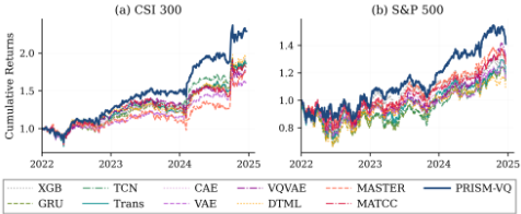
Table 1 summarizes performance on CSI 300 and S&P 500 over the 2022-2024 test period. On CSI 300, PRISM-VQ achieves a RankIC of 0.0646 and an SR of 1.57, outperforming all baselines, including DTML and GRU. It also attains the highest annualized return with a low MDD. On S&P 500, PRISM-VQ reaches a RankIC of 0.0141 and an SR of 0.67, with the lowest MDD of 0.1616, representing a 58.4% RankIC improvement over DTML. Statistical significance is evaluated on daily RankIC using a block bootstrap test with 10K resamples. PRISM-VQ significantly outperforms competing methods in 17 of 20 baseline comparisons across both markets at the p < 0.05 level. These results demonstrate consistent improvements in ranking accuracy and portfolio performance across market regimes, as further illustrated by cumulative returns in Figure 3.
| CSI 300 | S&P 500 | |||
|---|---|---|---|---|
| Configuration | RankIC | RankICIR | RankIC | RankICIR |
| Full Model | 0.0646 | 0.4224 | 0.0141 | 0.1208 |
| w/o Prior | 0.0548 | 0.3756 | 0.0031 | 0.0314 |
| w/o MoE | 0.0586 | 0.3958 | 0.0081 | 0.0736 |
| w/o Codebook | 0.0472 | 0.2938 | -0.0024 | -0.0179 |
5.3 Ablation Study (RQ2)
Table 2 evaluates the contribution of three core components of PRISM-VQ: expert prior factors (fp), structure-conditioned MoE routing, and the discrete codebook. Removing the codebook causes the largest degradation, with RankIC dropping by 26.9% on CSI 300 and becoming negative on S&P 500, highlighting the importance of discrete latent structure. Excluding prior factors reduces RankIC by 15.2% and 78.0% on CSI 300 and S&P 500, confirming the regularizing role of expert knowledge. Replacing MoE with a single network lowers RankIC by 9.3% and 42.6%, confirming the necessity of structure-conditioned temporal modeling. The consistently larger degradation on S&P 500 suggests all three components act synergistically to extract weak signals in efficient markets, whereas CSI 300's stronger signal environment allows partial compensation.
| CSI 300 | S&P 500 | |||||||||||
|---|---|---|---|---|---|---|---|---|---|---|---|---|
| K=40 | K=40 | K=50 | ||||||||||
| Model | AR | MDD | SR | AR | K=50 MDD | SR | AR | MDD | SR | AR | MDD | SR |
| XGB | 0.22 | 0.22 | 1.11 | 0.19 | 0.22 | 0.97 | 0.11 | 0.20 | 0.45 | 0.10 | 0.20 | 0.42 |
| GRU | 0.20 | 0.23 | 1.09 | 0.19 | 0.23 | 1.05 | 0.08 | 0.30 | 0.35 | 0.07 | 0.28 | 0.30 |
| TCN | 0.22 | 0.21 | 1.19 | 0.21 | 0.21 | 1.15 | 0.10 | 0.24 | 0.43 | 0.10 | 0.25 | 0.46 |
| Trans | 0.24 | 0.23 | 1.19 | 0.20 | 0.23 | 1.03 | 0.08 | 0.28 | 0.35 | 0.08 | 0.27 | 0.35 |
| CAE | 0.03 | 0.21 | 0.17 | 0.04 | 0.22 | 0.19 | 0.08 | 0.21 | 0.42 | 0.08 | 0.20 | 0.44 |
| VAE | 0.19 | 0.19 | 1.08 | 0.17 | 0.20 | 0.97 | 0.09 | 0.24 | 0.47 | 0.11 | 0.22 | 0.54 |
| VQVAE | 0.20 | 0.19 | 1.02 | 0.17 | 0.19 | 0.91 | 0.09 | 0.20 | 0.45 | 0.09 | 0.21 | 0.47 |
| DTML | 0.02 | 0.22 | 0.12 | 0.03 | 0.22 | 0.15 | 0.07 | 0.19 | 0.39 | 0.06 | 0.19 | 0.36 |
| MASTER | 0.19 | 0.26 | 0.81 | 0.18 | 0.25 | 0.77 | 0.10 | 0.21 | 0.44 | 0.10 | 0.22 | 0.43 |
| MATCC | 0.19 | 0.24 | 0.92 | 0.18 | 0.24 | 0.86 | 0.11 | 0.21 | 0.51 | 0.10 | 0.22 | 0.47 |
| PRISM-VQ | 0.28 | 0.18 | 1.48 | 0.25 | 0.20 | 1.37 | 0.14 | 0.16 | 0.67 | 0.12 | 0.16 | 0.61 |
5.4 Robustness Analysis (RQ3)
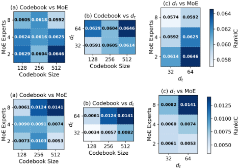
Model hyperparameters. Figure 4 shows sensitivity to the codebook size K, temporal dimension dt, and number of experts Me. Across both markets, performance peaks at dt = 64 and K = 512, indicating that moderate temporal capacity with fine-grained quantization is optimal. The optimal number of experts differs by market: CSI 300 peaks at Me = 2, while S&P 500 improves up to Me = 8, suggesting that more efficient markets benefit from greater expert specialization. The shared optimum at K = 512 indicates that fine-grained discrete quantization is broadly beneficial.
Portfolio size. Table 3 reports performance for larger TopK portfolios (K ∈ {40, 50}). PRISM-VQ consistently outperforms all baselines, achieving an AR of 27.85% and 25.35% on CSI 300 and 13.96% and 12.42% on S&P 500 for K=40 and K=50, respectively, representing improvements of 17-27% over the strongest baselines. PRISM-VQ also attains the lowest MDD on S&P 500 across all settings (15.8216.07%), while gradual performance degradation with larger K indicates robust signals beyond top-ranked stocks. 5
5 Additional robustness results under varying transaction costs are available in Technical Appendix E of the extended version.
| Top 3 Factors | ρ | ||||||
|---|---|---|---|---|---|---|---|
| Market | Code | F1 | F2 | F3 | ρ1 | ρ2 | ρ3 |
| S&P | 72 34 224 | Prof. Qual. Prof. | LowRisk Size LowLev. | Mom. Prof. LowRisk | +.118 -.113 -.113 | +.109 +.097 +.112 | +.096 -.077 -.110 |
| CSI | 482 247 179 | Qual. LowLev. Size | Accr. Value Prof. | Invest. Invest. Qual. | -.118 -.117 +.117 | +.115 +.117 -.081 | +.113 +.103 -.077 |
5.5 Interpretation of Representations (RQ4)
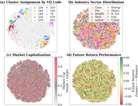
Visualization of learned representations. Figure 5 presents a t-SNE visualization of learned discrete representations on the S&P 500 in 2024. 6 The ten most frequent codes form well-separated clusters (panel (a)), yet stocks from different sectors are substantially mixed across clusters (panel (b)), indicating that vector quantization captures structure beyond sector taxonomies encoded by prior factors. While larger-cap and positive-return stocks tend to concentrate in certain regions (panels (c)-(d)), the lack of clear separation suggests the codes capture a richer cross-sectional structure not driven solely by market capitalization or future returns.
Factor exposure analysis. Economic interpretability is evaluated via Spearman correlations between code-specific returns and 13 JKP factor returns (Table 4). The codes exhibit systematic but moderate factor associations (e.g., S&P 500 Code 72 loads on profitability, low-risk, and momentum, consistent with a quality-growth profile) with maximum correlations of approximately 0.12, indicating multi-dimensional factor combinations rather than the replication of individual factors. The codes also show temporal stability, with monthly persistence rates of 4.9% on CSI 300 and 7.4% on S&P 500, substantially exceeding the 1% uniform baseline. 7
6 The list of representative stocks is available in Technical Appendix G of the extended version.
5.6 Expert Specialization (RQ5)
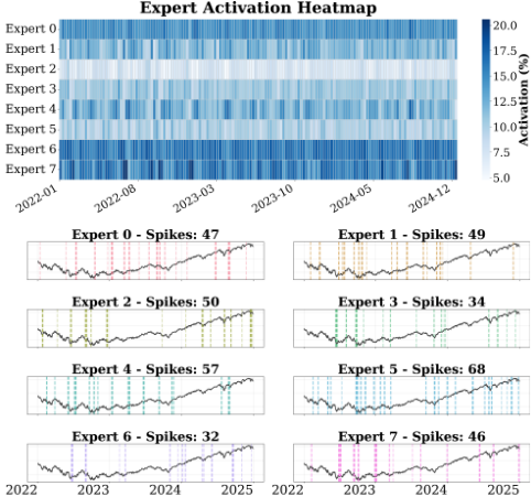
Figure 6 shows the MoE routing on the S&P 500. The top heatmap reveals heterogeneous expert utilization: Experts 6 and 7 dominate with approximately 16-20% average activation, while Expert 2 remains sparse at around 5-7%.
Regime-dependent timing is examined in the bottom panel, which visualizes daily activation spikes computed from the mean gating weight Pe,t = 1 Nt ∑Nt i=1 Gi,e,t, consistent with Eq.(23). Spikes are identified when Pe,t exceeds µe + 1.5σe. Pairwise Wilcoxon signed-rank tests across all 28 expert pairs indicate statistically distinct activation distributions, with all p-values below 0.001. The strongest separation occurs between Expert 2 (mean activation 7.09%) and Expert 6 (mean activation 16.46%). Expert 2 functions as a rare specialist that activates in specific market regimes, whereas Expert 6 remains consistently engaged.
Low overlap in spike dates further supports temporal specialization. The Jaccard overlap is 6.8%, compared to an 8.11% baseline, indicating that experts respond to distinct market conditions rather than activating synchronously.
6 Conclusion
We proposed PRISM-VQ, a two-stage framework for crosssectional stock rank prediction that learns reusable discrete cross-sectional structure via vector quantization with contrastive regularization and generates time-varying factor loadings through structure-conditioned MoE routing guided by financial priors. Across CSI 300 and S&P 500, PRISM-VQ consistently improves prediction and portfolio performance over strong baselines while producing interpretable discrete codes and specialized expert behaviors. These results indicate that combining a discrete information bottleneck with priorinformed conditional computation is an effective design principle for low-SNR, non-stationary financial return prediction problems.
Acknowledgments
This work was supported by the National Research Foundation of Korea (NRF) grant funded by the Korea government (MSIT) (No. RS-2025-24803415). The authors gratefully acknowledge the support provided by RiskX Corp.
@inproceedings{ijcai2026p492,
  title     = {Vector-Quantized Discrete Latent Factors Meet Financial Priors: Dynamic Cross-Sectional Stock Ranking Prediction for Portfolio Construction},
  author    = {Kim, Namhyoung and Song, Jae Wook},
  booktitle = {Proceedings of the Thirty-Fifth International Joint Conference on
               Artificial Intelligence, {IJCAI-26}},
  publisher = {International Joint Conferences on Artificial Intelligence Organization},
  editor    = {Diego Calvanese},
  pages     = {4421--4429},
  year      = {2026},
  month     = {8},
  note      = {Main Track},
  doi       = {10.24963/ijcai.2026/492},
  url       = {https://doi.org/10.24963/ijcai.2026/492},
}
TY - CPAPER TI - Vector-Quantized Discrete Latent Factors Meet Financial Priors: Dynamic Cross-Sectional Stock Ranking Prediction for Portfolio Construction AU - Kim, Namhyoung AU - Song, Jae Wook T2 - Proceedings of the Thirty-Fifth International Joint Conference on Artificial Intelligence, IJCAI-26 PB - International Joint Conferences on Artificial Intelligence Organization PY - 2026 SP - 4421 EP - 4429 DO - 10.24963/ijcai.2026/492 UR - https://doi.org/10.24963/ijcai.2026/492 ER -Copied
Machine-readable versions of this paper, for tools and AI agents:





