
Learning to Price and Stock Under Contextual and Censored Demand
Proceedings of the Thirty-Fifth International Joint Conference on Artificial Intelligence. Main Track. Pages 4339-4347.
https://doi.org/10.24963/ijcai.2026/483
Keywords
- Machine Learning: Multi-armed bandits
- Machine Learning: Online learning
- Machine Learning: Learning theory
- Machine Learning: Model-based and model learning reinforcement learning
Abstract
To make optimal joint pricing and inventory control decisions is a critical challenge for modern retailers. In practice, retailers face changing market conditions where demands are influenced by various contextual factors, while simultaneously dealing with the difficulty of lost sales that obscure true demand information. However, existing approaches often fail to account for both contextual information and censored demand observations. We address this gap by presenting a framework where we model demand as a linear combination of basis functions with unknown coefficients, allowing for adaptive pricing and inventory decisions that respond to changing contexts. We propose an efficient algorithm to achieve regret bound O(K sqrt(T) log T) under concave revenue conditions and O(K^(2/3) T^(2/3) (log T)^(1/2)) for the general case, with matching lower bounds confirming optimality. Extensive numerical experiments across diverse scenarios demonstrate our algorithm’s effectiveness.
- [Abbasi-Yadkori et al., 2011] Yasin Abbasi-Yadkori, Dávid Pál, and Csaba Szepesvári. Improved algorithms for lin- ear stochastic bandits. Advances in neural information processing systems, 24, 2011.
- [Agarwal et al., 2012] Alekh Agarwal, Miroslav Dudík, Satyen Kale, John Langford, and Robert Schapire. Contex- tual bandit learning with predictable rewards. In Artificial Intelligence and Statistics, pages 19-26. PMLR, 2012.
- [Auer, 2002] Peter Auer. Using confidence bounds for exploitation-exploration trade-offs. Journal of Machine Learning Research, 3(Nov):397-422, 2002.
- [Bensoussan et al., 2019] Alain Bensoussan, Yangyang Xie, and Houmin Yan. Joint inventory-pricing optimization with general demands: An alternative approach for concavity preservation. Production and Operations Management, 28(9):2390-2404, 2019.
- [Besbes and Zeevi, 2015] Omar Besbes and Assaf Zeevi. On the (surprising) sufficiency of linear models for dynamic pricing with demand learning. Management Science, 61(4):723-739, 2015.
- [Bu et al., 2022] Jinzhi Bu, David Simchi-Levi, and Chonghuan Wang. Context-based dynamic pricing with partially linear demand model. Advances in Neural Information Processing Systems, 35:23780-23791, 2022.
- [Cesa-Bianchi et al., 2019] Nicolo Cesa-Bianchi, Tommaso Cesari, and Vianney Perchet. Dynamic pricing with finitely many unknown valuations. In Algorithmic Learning Theory, pages 247-273. PMLR, 2019.
- [Chen and Simchi-Levi, 2012] Xin Chen and David Simchi- Levi. Pricing and Inventory Management. Oxford Univer- sity Press, United Kingdom, November 2012. Publisher Copyright: © Oxford University Press, 2013.
- [Chen et al., 2019] Boxiao Chen, Xiuli Chao, and Hyun-Soo Ahn. Coordinating pricing and inventory replenishment with nonparametric demand learning. Operations Research, 67(4):1035-1052, 2019.
- [Chen et al., 2021] Boxiao Chen, Xiuli Chao, and Cong Shi. Nonparametric learning algorithms for joint pricing and in- ventory control with lost sales and censored demand. Math- ematics of Operations Research, 46(2):726-756, 2021.
- [Chen et al., 2024] Boxiao Chen, Yining Wang, and Yuan Zhou. Optimal policies for dynamic pricing and inventory control with nonparametric censored demands. Manage- ment Science, 70(5):3362-3380, 2024.
- [Choi et al., 2023] Young-Geun Choi, Gi-Soo Kim, Choi Yunseo, Wooseong Cho, Myunghee Cho Paik, and Min- hwan Oh. Semi-parametric contextual pricing algorithm using cox proportional hazards model. In International Con- ference on Machine Learning, pages 5771-5786. PMLR, 2023.
- [Chu et al., 2011] Wei Chu, Lihong Li, Lev Reyzin, and Robert Schapire. Contextual bandits with linear payoff functions. In Proceedings of the Fourteenth International Conference on Artificial Intelligence and Statistics, pages 208-214. JMLR Workshop and Conference Proceedings, 2011.
- [Cohen et al., 2020] Maxime C Cohen, Ilan Lobel, and Re- nato Paes Leme. Feature-based dynamic pricing. Manage- ment Science, 66(11):4921-4943, 2020.
- [Ding et al., 2021] Jingying Ding, Woonghee Tim Huh, and Ying Rong. Feature-based nonparametric inventory control with censored demand. Social Science Research Network, 2021.
- [Fan et al., 2024] Jianqing Fan, Yongyi Guo, and Mengxin Yu. Policy optimization using semiparametric models for dynamic pricing. Journal of the American Statistical Asso- ciation, 119(545):552-564, 2024.
- [Foster and Rakhlin, 2020] Dylan Foster and Alexander Rakhlin. Beyond ucb: Optimal and efficient contextual ban- dits with regression oracles. In International Conference on Machine Learning, pages 3199-3210. PMLR, 2020.
- [Foster et al., 2018] Dylan Foster, Alekh Agarwal, Miroslav Dudík, Haipeng Luo, and Robert Schapire. Practical contex- tual bandits with regression oracles. In International Con- ference on Machine Learning, pages 1539-1548. PMLR, 2018.
- [Golrezaei et al., 2019] Negin Golrezaei, Adel Javanmard, and Vahab Mirrokni. Dynamic incentive-aware learning: Robust pricing in contextual auctions. Advances in Neural Information Processing Systems, 32, 2019.
- [Gong and Zhang, 2024] Xueping Gong and Jiheng Zhang. Minimax optimality in contextual dynamic pricing with general valuation models. arXiv preprint arXiv:2406.17184, 2024.
- [Huh and Rusmevichientong, 2009] Woonghee Tim Huh and Paat Rusmevichientong. A nonparametric asymptotic anal- ysis of inventory planning with censored demand. Mathe- matics of Operations Research, 34(1), 2009.
- [Javanmard and Nazerzadeh, 2019] Adel Javanmard and Hamid Nazerzadeh. Dynamic pricing in high-dimensions. Journal of Machine Learning Research, 20(9):1-49, 2019.
- [Lattimore and Szepesvári, 2020] Tor Lattimore and Csaba Szepesvári. Bandit algorithms. Cambridge University Press, 2020.
- [Li et al., 2017] Lihong Li, Yu Lu, and Dengyong Zhou. Prov- ably optimal algorithms for generalized linear contextual bandits. In International Conference on Machine Learning, pages 2071-2080. PMLR, 2017.
- [Lin et al., 2022] Meichun Lin, Woonghee Tim Huh, Harish Krishnan, and Joline Uichanco. Data-driven newsvendor problem: Performance of the sample average approxima- tion. Operations Research, 70(4):1996-2012, 2022.
- [Luo et al., 2022] Yiyun Luo, Will Wei Sun, and Yufeng Liu. Contextual dynamic pricing with unknown noise: Explore- then-ucb strategy and improved regrets. Advances in Neural Information Processing Systems, 35:37445-37457, 2022.
- [Luo et al., 2024] Yiyun Luo, Will Wei Sun, and Yufeng Liu. Distribution-free contextual dynamic pricing. Mathematics of Operations Research, 49(1):599-618, 2024.
- [Lyu et al., 2024] Jiameng Lyu, Jinxing Xie, Shilin Yuan, and Yuan Zhou. A minibatch stochastic gradient descent-based learning metapolicy for inventory systems with myopic optimal policy. Management Science, 2024.
- [Petruzzi and Dada, 1999a] Nicholas C. Petruzzi and Maq- bool Dada. Pricing and the news vendor problem: a review with extensions. Oper. Res., 47(2):183-194, February 1999.
- [Petruzzi and Dada, 1999b] Nicholas C Petruzzi and Maq- bool Dada. Pricing and the newsvendor problem: A re- view with extensions. Operations research, 47(2):183-194, 1999.
- [Qin et al., 2022] Hanzhang Qin, David Simchi-Levi, and Li Wang. Data-driven approximation schemes for joint pricing and inventory control models. Management Sci- ence, 68(9):6591-6609, 2022.
- [Shi et al., 2016] Cong Shi, Weidong Chen, and Izak Duenyas. Nonparametric data-driven algorithms for multi- product inventory systems with censored demand. Opera- tions Research, 64(2):362-370, 2016.
- [Simchi-Levi and Xu, 2021] David Simchi-Levi and Yun- zong Xu. Bypassing the monster: A faster and simpler optimal algorithm for contextual bandits under realizability. Mathematics of Operations Research, 2021.
- [Takemura et al., 2021] Kei Takemura, Shinji Ito, Daisuke Hatano, Hanna Sumita, Takuro Fukunaga, Naonori Kakimura, and Ken-ichi Kawarabayashi. A parameter- free algorithm for misspecified linear contextual bandits. In International Conference on Artificial Intelligence and Statistics, pages 3367-3375. PMLR, 2021.
- [Wang et al., 2021a] Hanzhao Wang, Kalyan Talluri, and Xi- aocheng Li. On dynamic pricing with covariates. arXiv preprint arXiv:2112.13254, 2021.
- [Wang et al., 2021b] Yining Wang, Boxiao Chen, and David Simchi-Levi. Multimodal dynamic pricing. Management Science, 67(10):6136-6152, 2021.
- [Whitin, 1955] Thomson M Whitin. Inventory control and price theory. Management science, 2(1):61-68, 1955.
- [Xu and Wang, 2022] Jianyu Xu and Yu-Xiang Wang. To- wards agnostic feature-based dynamic pricing: Linear poli- cies vs linear valuation with unknown noise. In Interna- tional Conference on Artificial Intelligence and Statistics, pages 9643-9662. PMLR, 2022.
- [Yano and Gilbert, 2004] Candace A. Yano and Stephen M. Gilbert. Coordinated Pricing and Production/Procurement Decisions: A Review, pages 65-103. Springer US, Boston, MA, 2004.
- [Zhang et al., 2020] Huanan Zhang, Xiuli Chao, and Cong Shi. Closing the gap: A learning algorithm for lost-sales inventory systems with lead times. Management Science, 66(5):1962-1980, 2020.
References were extracted automatically from the PDF and may contain errors.
Full text extracted automatically from the PDF; figures, tables and equations may differ. The PDF is the version of record.
1 Introduction
In recent years, joint pricing and inventory control has gained significant attention from both academia and industry. Leading retailers increasingly leverage data science to drive innovation in pricing strategies, inventory management, and supply chain optimization. This growing interest is reflected in comprehensive surveys [Chen and Simchi-Levi, 2012; Yano and Gilbert, 2004; Petruzzi and Dada, 1999a]. However, a critical gap remains: most existing models overlook the role of censored demand and contextual information, which are essential for adaptive decision-making. In this paper, we address this gap by studying the optimal joint pricing and inventory control strategy with lost sales that incorporates contextual information, aiming to bring theory closer to real-world applications.
In this paper, we study a joint pricing and inventory control problem with contextual information and lost sales over a finite horizon of T periods. At the start of each period, the seller observes contextual information that influences customer demand. The demand function is modeled as a linear combination of K basis functions with unknown coefficients, plus an independent random noise term. Using the observed context and an estimated demand function, the seller simultaneously sets the selling price and inventory level, with replenishment taking effect immediately. After making the decisions, only the censored demand, i.e., the minimum between actual demand and available inventory, is observed as unmet demand are lost. Leftover inventory carries over to the next period, incurring a linear holding cost, while unmet demand results in a linear lost penalty cost. The objective is to maximize profit, defined as sales revenue minus inventory holding and lost sales costs, across the T-period horizon.
∗Corresponding author.
Our problem introduces several interconnected challenges that complicate both theoretical analysis and practical implementation. First, the presence of censored demand obstructs direct observation of true demand signals, necessitating the development of unbiased estimators for the demand function while mitigating inherent biases from incomplete data. Second, the inclusion of contextual factors result in the problem being dynamic, thus traditional optimization methods which lead to static policies become inapplicable. Both the pricing and inventory decisions must adapt to contextual information in order to achieve optimality. Finally, when applying our methodology to models beyond the combination of the basis functions, approximation errors arise due to structural mismatches between idealized model and real-world dynamics, demanding rigorous error quantification and robustness guarantees. Together, these challenges necessitate a novel integration of censored data correction, context-aware online optimization, stochastic inventory control, and error-bounded approximation techniques.
Our contributions can be summarized as followings:
- Context-Aware Pricing and Inventory Optimization. We propose a framework for joint pricing and inventory management (see Table 1) where decisions adapt to contextual information, with both pricing and inventory policies responding to changing contexts.
- Algorithmic Framework and Regret Analysis. We propose an easy-to-implement algorithm addressing censored demand, dynamic contexts, and stochastic inventory dynamics. Under concave revenue,
| Paper | Context | Censored Demand | Upper Bound | Lower Bound | Assumptions |
|---|---|---|---|---|---|
| [Chen et al., 2019] | No | No | √T | N/A | - |
| [Chen et al., 2021] | No | Yes | T 1 2 +ν | N/A | √logT-differentiable, concave |
| [Chen et al., 2024] | No | Yes | √T | N/A | Twice-differentiable, concave |
| [Chen et al., 2024] | No | Yes | T 35 | T 3 5 | Twice-differentiable |
| Ours | Yes | Yes | T 23 | T 2 3 | Differentiable |
| Ours | Yes | Yes | √T | N/A | Twice-differentiable, concave |
Note: The regrets listed above omit constant factors and poly(logT) terms. Here, ν = 1 √3 lnT + 0.25 √lnT .
Table 1. Comparison of Regret Bounds under Joint Pricing and Inventory Control Problems
our method achieves O(K√T logT) regret, matching the lower bound. Without concavity, we derive O(K2/3T 2/3 (log T)1/2 ) regret and prove a lower bound Ω(T (m+1)/(2m+1) ) in Theorem 4.4 for m-th differentiable revenue functions, establishing minimax optimality (see Table 1).
- Inventory Feasibility. To address infeasible target inventory levels from contextual information, we develop a queueing-theoretic method using stochastic recursion to bound regret from inventory mismatches, ensuring stable performance under stochasticity.
1.1 RelatedWork
Dynamic pricing. Initial research focused on non-contextual dynamic pricing [Besbes and Zeevi, 2015; Cesa-Bianchi et al., 2019]. Wang et al. [2021b] achieved ˜O(T (m+1)/(2m+1) ) regret for m-th smooth demand functions with matching lower bounds. Bu et al. [2022] extended this to additive linear contextual effects, establishing instance-dependent bounds. Other models assume Bernoulli purchase decisions [Javanmard and Nazerzadeh, 2019; Golrezaei et al., 2019; Choi et al., 2023; Xu and Wang, 2022; Luo et al., 2024; Luo et al., 2022; Fan et al., 2024]. Related studies [Luo et al., 2024; Luo et al., 2022; Fan et al., 2024] share similar settings but differ in noise distribution assumptions, with regret bounds ranging from ˜O(d20T 2/3 ) to ˜O((d0T)(2m+1)/(4m-1) ) [Luo et al., 2022; Fan et al., 2024]. Gong and Zhang [2024] achieved ˜O(d1/3 0 T 2/3 ) with minimax optimality.
Inventory control. Classical inventory models, such as the newsvendor model [Petruzzi and Dada, 1999b], assume i.i.d. demand and use SGD-based methods for optimization, extended to multi-product settings, delayed replenishment [Zhang et al., 2020], and quantity constraints [Shi et al., 2016]. Lyu et al. [2024] addressed SGD infeasibility using mini-batch strategies. Recent work incorporates demand characteristics [Ding et al., 2021], while SAA methods construct empirical distributions from demand samples [Lin et al., 2022].
Joint pricing and inventory control. Whitin [1955] first introduced joint pricing and inventory control with full information. Subsequent work [Bensoussan et al., 2019] used dynamic programming, while Qin et al. [2022] proposed approximations with sample complexity analysis. In online learning settings, Chen et al. [2019] considered data-driven models without historical data. Chen et al. [2021] addressed censored demand using spline interpolation and sample average methods. Chen et al. [2024] proposed ternary/binary search methods for convex/non-convex demand functions, establishing theoretical lower bounds. However, existing models ignore contextual information; once contexts are considered, optimal prices and inventory change over time, making prior algorithms inapplicable. We summarize comparisons in Table 1.
Contextual bandit. Our policy connects to bandit algorithms [Lattimore and Szepesvári, 2020; Foster and Rakhlin, 2020; Abbasi-Yadkori et al., 2011; Takemura et al., 2021; Auer, 2002; Simchi-Levi and Xu, 2021], including linear [Abbasi-Yadkori et al., 2011] and generalized linear bandits [Li et al., 2017; Chu et al., 2011]. Recent work [Foster et al., 2018; Agarwal et al., 2012; Foster and Rakhlin, 2020] achieved optimal regret bounds for general function classes with regression oracles.
Notations. Throughout the paper, we use the following notations. For any positive integer n, we denote the set {1, 2, · · · , n} as [n]. The cardinality of a set A is denoted by |A|. We use I{E} to represent the indicator function of the event E. Specifically, I{E} takes the value 1 if E happens, and 0 otherwise. For norms, we utilize the notation ∥ · ∥p where 1 ≤ p ≤ ∞ to denote the ℓp norm. Throughout the analysis, the notation ˜O is employed to hide the dependence on absolute constants and logarithmic terms. It allows us to focus on the dominant behavior of the quantities involved.
2 Basic Setting
Consider a company selling a single type of products over a time period of T rounds. At the beginning of each round t, the firm observes a context xt drawn i.i.d. from an unknown distribution in a compact domain X. Using this context, the company determines a pricing pt and inventory order-up-to decision yt. The demand is modeled as Dt = λ(xt, pt) + ϵt, where λ(·, ·) is a deterministic function capturing the demandcontext-price curve, and ϵt is an i.i.d. noise random variable with mean 0. The distribution function and density function of ϵt are denoted as F and f, respectively. The company has no prior knowledge of the function λ(·, ·) or the distribution F, and it must make its pricing and inventory decisions sequentially, relying solely on historical data to maximize the T period total profit.
Decision dynamics. Let It denote the inventory level before replenishment at the start of the round t. An admissible policy is represented by {(pt, yt), t ≥ 1}, where pt ∈ [pmin, pmax] is the price, and yt ≥ It is the order-up-to inventory level. The decision (pt, yt) depends only on the observable contexts and historical data prior to the round t.
Given any admissible policy {(pt, yt), t ≥ 1}, the sequence of events for each round t is described as follows:
- At the beginning of each round t, the firm observes the context xt ∈ X ⊆ Rd and the starting inventory level It.
- The firm decides to place an order to bring the inventory level up to yt ≥ It, and also sets the selling price pt ∈ [pmin, pmax]. We assume that newly ordered items arrive instantly, meaning that the ordering lead time is zero.
- The demandDt realizes and is satisfied up to the available inventory. Any unsatisfied demand is lost and unobservable. Therefore, the lost-sales quantity (Dt -yt)+ is not observable, and the firm only observes the sales quantity (censored demand) ot = min{Dt, yt}, rather than the full realized Dt.
- At the end of round t, the firm incurs a profit of
where h and b are the per-unit holding and lost-sales penalty costs, respectively.
- Products may be perishable, with an unknown perishability rate ρ ∈ [0, 1], which impacts the inventory carried over to the next period. The state transition is given by
Full information benchmark. The firm's goal is to maximize the T -period expected total profit ∑Tt=1 E[qt], by constructing an admissible policy {(pt, yt), t ≥ 1}. This is a fundamental model for joint pricing and inventory control, with potential applications in various realistic retail scenarios.
Assuming the demand curve λ(·, ·) and noise distribution F are known, we define the myopic pricing and replenishment policy as a benchmark. This policy is represented as
The regret at time t is defined as the loss in reward resulting from setting the price pt and the inventory level yt compared to the optimal price and inventory level. The cumulative regret over the horizon of T periods, denoted as R(T), is given by the expression:
To assess performance, we consider the expected cumulative regret E[R(T)], which accounts for the randomness in covariates and the potential randomness in the pricing policy.
Assumptions. We make the following assumptions, most of which are rather standard in the literature.
First, we consider the linear additive model as the demand function, which means that λ(x, p) is a linear combination of the basis function.
Assumption 1. There exists a set of basis functions {λi(x, p)}Ki=1 and a unique unknown parameter θ∗ = (θ∗ 1 , θ∗ 2 , · · · , θ∗K )⊤ such that λ(x, p) = ∑Ki=1 θ∗ i λi(x, p).
This assumption includes many commonly used demand functions, such as [Cohen et al., 2020]. Next, we introduce some basic assumptions on the revenue function.
Assumption 2. The revenue function Q(x, p, y) is continuously differentiable with respect to x, p and y.
The differentiability of Q is a common assumption in the literature, as seen in works such as [Chen et al., 2019; Qin et al., 2022; Chen et al., 2024]. For the dynamic pricing component, this assumption is particularly relevant, as it encompasses many practical demand functions, including those discussed in [Cohen et al., 2020; Wang et al., 2021b; Wang et al., 2021a]. In inventory control, several papers, such as [Shi et al., 2016; Ding et al., 2021], adopt the newsvendor objective function, which is differentiable with respect to the inventory level y. These properties are crucial for deriving closed-form solutions for the optimal inventory level y∗ (x, p) given the context x.
Proposition 1. The optimal inventory level enjoys the following structure: y∗ (x, p) = λ(x, p) + z∗ (p), where z∗ (p) = F -1 Ä b+p b+p+h ä.
A context-free version of this result has appeared in [Ding et al., 2021; Chen et al., 2021; Chen et al., 2024]. To extend this to contextual dynamic pricing, we follow the process outlined below. To obtain the optimal inventory level. We begin by noting that ∂Q ∂y = b+p-(b+p+h)F(y-λ(x, p)). The optimal order-up-to level thus is given by y∗ (x, p) = λ(x, p) + z∗ (p), where z∗ (p) satisfies z∗ (p) = F -1 Ä b+p b+p+h ä . Finally, we assume some basic properties of the distribution noise, which is rather standard in the literature.
Assumption 3. The random error ϵt is bounded on the interval [ϵ, ϵ], and there exist positive constants κ1 and κ2 such that for any p ∈ [pmin, pmax] and ϵ0 ∈ îF -1 Ä b+p b+p+h ä -κ1, F -1 Ä b+p b+p+h ä + κ1 ó, we have f (ϵ0) ≥ κ2.
The first assumption on ϵt ensures the boundedness of the demand, which is a mild and common assumption in realworld applications [Chen et al., 2024]. It is important to note that we do not require the decision maker to know the exact bounds of the noise or the demand function. The second assumption is satisfied by many continuous random variables, including uniform and truncated Gaussian distributions. And the third assumption needs the demand to be larger than a certain range of the noise ensuring robustness. In the following sections, we propose our algorithm and further discuss the approximation error of the demand function.
3 AlgorithmDesign
We present our algorithmic design and summarize the key challenges in this setting.
The first challenge is censored demand: lost sales are unobservable, so we cannot directly estimate the true demand parameter θ∗ . To mitigate this, we set the inventory level to scale with logT, improving demand observability without knowing the true demand upper bound.
The second challenge is the period-varying optimal inventory level due to changing contexts and perishable inventory constraints, which may make the ideal up-to-order level infeasible. We address this using a queue-based approach to control deviations from the recommended target inventory.
Recall from proposition 1 that the optimal inventory level is y∗ (x, p) = λ(x, p) + z∗ (p), where z∗ (p) is the safety stock level. The corresponding revenue function is
where x is the context and p is the price. The decision-maker estimates G(x, p) to determine the optimal price and then computes the corresponding target inventory.
Our method splits the time horizon into two phases: exploration and commitment. During exploration, we sample prices uniformly at random and set the inventory level high enough to fully observe demand, avoiding censoring and ensuring reliable feedback. The inventory level is tuned to balance learning accuracy and regret. We estimate the demand function using least-squares, leveraging the linear structure of the basis functions. Least-squares is chosen because its estimation error is negligible compared to the overall regret. Next, we estimate the total cost (including lost-sales and holding costs) by accurately estimating the optimal inventory function z(p) and the residual error. We approximate the demand distribution empirically and compute z(p) via the inverse CDF. With these estimates, we construct an empirical revenue function. Overall, our algorithm is simple, efficient, and practical for joint pricing and inventory control under censored demand and perishable constraints.
4 Regret Analysis
The main result of this section is that the proposed algorithm converges to the full information benchmark at a rate of O(K√T log T) under the strongly concave assumption, and at a rate of O(K2/3T 2/3 (log T)1/2 ) without this assumption. We provide a detailed regret analysis in the following two subsections.
4.1 Strongly Concave Revenue Function
In this subsection, we present several additional assumptions that are standard in the literature (e.g., [Chen et al., 2021], [Chen et al., 2024], [Bensoussan et al., 2019]). These assumptions are crucial for establishing the theoretical framework and ensuring the robustness of our model.
Algorithm 1 Joint Pricing and Inventory Control Algorithm with Censored Demand
Input: the time horizon T , the length of the exploration phase T0, cost parameter h and b, basis function ϕ(x, p) = (λ1(x, p), λ2(x, p), · · · , λK(x, p))⊤
- 1: for round t = 1, 2, 3, · · · , T0 do
- 2: Observe a context xt and current inventory level It
- 3: Uniformly choose pt ∈ [pmin, pmax]
- 4: Set the inventory level yt = logT
- 5: Observe the sale ot =min{Dt, yt}
- 6: Estimate the parameter θ∗ by
- 7: Collect the samples for residuals ηt = ot - ˆ θ⊤ϕ(xt, pt) with t ∈ [T0]
- 8: Estimate the distribution F as
- 9: Estimate the quantity z(p) as
- 10: Construct the function ˆG(x, p) using:
- 11: for round t = T0 +1, T0 +2, · · · , T do
- 12: Observe a context xt and current inventory level It
- 13: Set pt ∈ argmax ˆG(xt, p)
- 14: Set the inventory level yt = (ˆ θ⊤ϕ(xt, pt)+ˆ z(pt))∨It
- 15: Observe the sale ot =min{Dt, yt}
First, we assume that the full information optimal price p∗t lies in the interior of the price interval [pmin, pmax] for any time t. This assumption is necessary to ensure that optimal pricing decisions can be made without hitting the boundaries of the price range, which could limit the effectiveness of pricing strategies.
Assumption 4. The full information optimal price p∗t lies in the interior of [pmin, pmax] for any t.
Building on this, we further assume that the function G(x, p), which represents the relationship between the state variable x and price p, is strongly concave in p for any given x. This concavity condition is crucial, as it guarantees that the revenue generated from pricing is maximized, leading to unique optimal pricing strategies. Specifically, there exists a parameter κ3 > 0 such that the second derivative of G with respect to p is always less than or equal to -κ3.
Assumption 5. G(x, p) is strongly concave in p for any x.
In other words, there exists a parameter κ3 > 0 such that ∂ 2 p G(x, p) ≤ -κ3 for any x.
Additionally, we require that the revenue function Q(x, p, y) is twice continuously differentiable with respect to the variables x, p, and y. This differentiability condition facilitates the application of optimization techniques and allows for smooth adjustments in response to changes in the underlying variables, ensuring a well-behaved revenue landscape.
Assumption 6. The revenue function Q(x, p, y) is twice continuously differentiable with respect to p, and y and continuous with respect to x.
Together, these assumptions create a robust foundation for analyzing the optimal pricing strategies within our model, ensuring both theoretical validity and practical applicability.
Now we are ready to give a sketch of proof of the Theorem 4.1: under strongly concave assumption. To give an upper bound on the regret, we first decompose the regret into the following terms:
where ˆ yt = ˆ θT ϕ(xt, pt) + ˆ z(pt) is the recommended inventory level and yt is the truly implemented inventory level.
Now we consider two separate situations regarding the demand model: the first is the linear additive model, while the second is the linear additive model with an approximation bias. We provide upper bounds for the four terms respectively under each demand model.
Theorem 4.1. Under Assumption 3, Assumption 1, Assumption 4, Assumption 5, Assumption 6, there exists a constant ˆ C such that the regret bound of our algorithm is R(T) ≤ ˆ CKT 12 logT.
In Equation (2), the first term represents the regret during the exploration phase, which increases linearly with the total duration of the exploration. In the exploitation phase, we decompose the regret into two terms, where ˆ y denotes the recommended inventory level and yt denotes the actual implemented inventory level. This decomposition is based on the fact that yt = max{It, ˆ yt}.
Using Taylor expansion, the second term in Equation (2) can be bounded as follows:
What remains is to bound the difference between the optimal price decision and the optimal inventory decision using the recommended strategy. By utilizing the strong concavity of the function G, we turn the difference of the price into the maximum of the differential of the function G:
Next, we need to bound the difference between the first derivative of the true function G and the empirical estimate ˆG, which can be bounded by the estimation error.
Similarly, the difference in inventory levels y∗ t - ˆ yt can be bounded using the definition and the bound of the price decision p∗t - pt. Thus, we have the following theorem:
Theorem4.2. In the exploitation phase, there exists a constant ˜ C such that
Finally, we need to provide an upper bound for the third term in Equation (2).
In the case It ≤ ˆ yt, we have yt = ˆ yt, which results in zero regret. Below, we only consider the case where It > ˆ yt:
Now we need to provide an upper bound on the difference yt - ˆ yt. To do this, we establish the connection between the contextual inventory level and the waiting time process. Unlike the method in [Chen et al., 2021], which considers a non-contextual setting with the same optimal decision across all periods, we need to bound the difference in inventory levels yt - ˆ yt dynamically.
To achieve this, we define the following two stochastic processes:
where
We have:
In the above stochastic processes, At serves as an intermediate process. Additionally, Bt can be interpreted as the waiting time of the t-th customer in the queuing system, where Jt is the interarrival time between the tth and (t + 1)-th customer, and ρq/√t is the service time for the tth customer.
This idea is similar to the method presented in [Huh and Rusmevichientong, 2009], which established a relationship between the amount of inventory exceeding the target level and the waiting time process in a GI/D/1 queue. However, they do not consider the impact of context and only need to bound the gradients to establish such a connection. In our analysis, since there are no gradients in the exploitation phase, we only need to exploit the estimation error during the exploration phase and the variability of features. Since this only involves the case where It > ˆ yt, this method is also robust to perishable inventory levels.
Proposition 4.1. For any t ≥ T0 + 1, yt - ˆ yt ≤ Bt with probability at least 1- 2 T 4 0 , where Bt is defined in Equation (6).
After providing a bound for the stochastic process defined above, we can upper bound the regret between the actual implemented inventory level and the recommended inventory level with the following proposition:
Proposition 4.2. There exists a constant C4 such that the regret from not achieving inventory targets during the commitment phase is bounded by E î∑Tt=T0+1 |Q(xt, pt, ˆ yt) -Q(xt, pt, yt)|ó ≤ C4T 12 which holds with probability at least 1 - 2 T 4 0 .
Summing up all the inequalities above, we can obtain the bound mentioned in Theorem 4.1.
4.2 Non-concave Revenue Function
The non-concave revenue function has been studied in Chen et al. [2024] in a non-contextual setting. They show that the penalty term related to inventory levels can destroy the concavity of the objective function, making the lost-sales model significantly more difficult to analyze compared to the backlogged case. To address this challenge, Chen et al. [2024] propose a search-based method for identifying the optimal price under the assumption that the revenue function is twice differentiable, with ˜Θ(T 3/5 ) minimax optimal regret bounds.
We extend their work in two key directions: we relax the assumption of second-order differentiability and generalize the problem to a contextual setting. In our case, the optimal prices vary over time due to changing contexts, and the revenue function G may lack smoothness, making the approach in Chen et al. [2024] inapplicable. Without assuming strong concavity of G, we are unable to derive a precise upper bound on the difference between successive price decisions, as was done in the previous section. Instead, we adopt a greedy strategy to control this difference, which leads to a regret bound that is worse than the O(K√T logT) rate achieved under more favorable assumptions.
Theorem 4.3. With Assumption 2 and Assumption 1, there exists a constant ˜ C such that the regret bound of our algorithm is R(T) ≤ ˜ CK 23 T 2 3 (log T ) 12 .
To prove Theorem 4.3, we decompose the regret into two parts:
- Bounding the revenue gap: G(xt, p∗t ) -G(xt, pt)
- Bounding the inventory regret: Q(xt, pt, y∗ t ) - Q(xt, pt, ˆ yt)
For the first part, we use a decomposition of G(xt, p∗t ) - G(xt, pt) and apply the estimation error bound for ˆG(xt, p), leading to:
For the second part, we use an existing result in Proposition 4.2 to bound the inventory regret term. Finally, combining these bounds results yields the desired results.
Theorem 4.4. For any policy π, there exists a non-contextual problem instance whose revenue function is m-th differentiable, such that R(T) ≥ Ω(T (m+1)/(2m+1) ) for sufficiently large T .
The instance construction is motivated by [Wang et al., 2021b]. The construction of the noise distribution starts with a smooth function u(x), which is normalized to define a function B(x), leading to a density function f(x) supported on [-1, 1] with mean 0. Using this, a demand function λj(p) is defined, which perturbs the base revenue function r0(p) using a small parameter η and a bump function. The reward function Qj(p, y) is shown to be m-th differentiable, with bounds on the Hellinger distance between different environments. A lower bound on expected regret is derived using the pigeonhole principle, showing that for some interval i∗ , the regret for any policy is at least Ω(T m+1 2m+1 ).
Combing the above upper and lower bounds, we conclude that Θ(T 23 ) is an achievable minimax optimal regret bounds only under the differentiabilty assumption.
5 Numerical Experiments
We conduct a numerical study to evaluate the empirical performance of our algorithms.
5.1 Test on parameters h and b
The experiments are based on a linear demand model:
where the parameter vector (α, β) ∈ R4 is sampled from a standard normal distribution and normalized to unit norm. The noise term ϵt is drawn independently from the uniform distribution over [-1, 1]. Prices are constrained to the range pmin = 0.1 and pmax = 2.
For each experimental setting, we perform 50 independent runs. At each round, context vectors xt are drawn from a standard normal distribution and normalized to unit length. We evaluate performance using relative regret, defined as R(T) T , where R(T) is the cumulative regret up to time T. Results are reported for time horizons T ∈ {100, 200, 500, 1000, 2000, 5000}, including the mean and standard deviation across trials.
The numerical experiments in Figure 1 show that relative regret decreases as the time horizon T increases. This trend holds across all three subplots with different parameter settings, indicating that the algorithm improves over time by leveraging more data for better decision-making and a balanced exploration-exploitation trade-off.
The error bars, representing standard deviation across trials, highlight increased variability at smaller T, due to insufficient data for reliable convergence. As T grows, the decreasing variability reflects improved stability. In Figure 2, the log-log plot shows a linear trend, suggesting a power-law relationship between regret and T, which supports the algorithm's robustness across different parameter settings.
5.2 Test on dimension K
We investigate how the algorithm's performance depends on the dimension of the basis functions, denoted by K. We vary K from 4 to 12 to assess its impact on regret. To ensure a fair comparison across different values of K, we fix the total time horizon at T = 1000, and set the cost parameters as h = 1 and b = 1. All other experimental settings remain consistent with the base configuration described earlier.
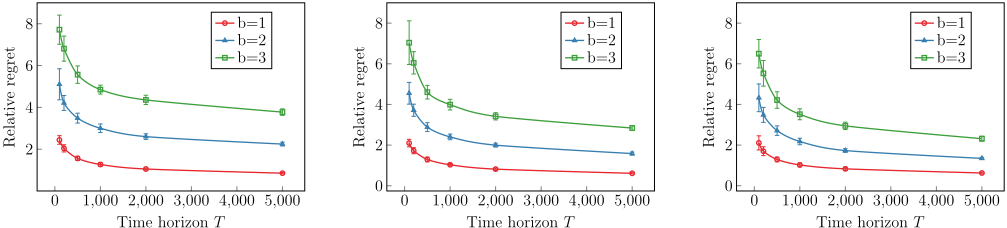
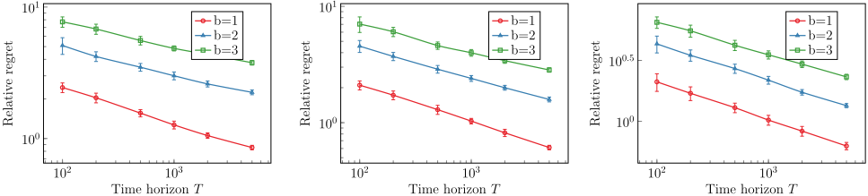
Figure 3 shows the relative regret across different K values. In summary, our results highlight key insights into the tradeoffs involved in contextual joint pricing and inventory control:
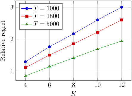
- Regret Increases with Model Complexity: The relative regret increases consistently with K, indicating that higher-dimensional models are more difficult to learn under a fixed time horizon. Intuitively, increasing K en-
- hances the expressive power of the model but requires more exploration.
- Stable Performance Across Trials: Despite the increased complexity, the algorithmmaintains controlled variance, with standard deviations remaining moderate across different values of K, indicating robust and reliable performance.
6 Conclusion
This paper studies the joint pricing and inventory control problem under a linear additive model with contextual information and censored demand observations. We address the critical gap where existing approaches fail to account for both contextual factors and the difficulty of lost sales that obscure true demand information.
Our main contributions include: (1) a context-aware framework for joint pricing and inventory management where both pricing and inventory policies adapt to changing contexts; (2) an easy-to-implement algorithm that achieves optimal regret bounds of O(K√T log T ) under concave revenue conditions and O(K2/3T 2/3 (log T )1/2 ) for the general case, with matching lower bounds confirming minimax optimality; and (3) a queueing-theoretic method to handle infeasible target inventory levels, ensuring stable performance under stochasticity. Extensive numerical experiments demonstrate the algorithm's effectiveness across diverse scenarios.
For future work, it would be valuable to investigate this problem under alternative modeling assumptions beyond the linear additive framework. It is also of interest to develop UCB-style analyses tailored to censored demand, which could offer principled exploration under partial observability.
Acknowledgments
This work was supported by the Theme-based Research Project T32-615/24-R and the General Research Fund 16500023 from the Hong Kong Research Grants Council.
@inproceedings{ijcai2026p483,
  title     = {Learning to Price and Stock Under Contextual and Censored Demand},
  author    = {Han, Zean and Ding, Zezhen and Zhang, Jiheng},
  booktitle = {Proceedings of the Thirty-Fifth International Joint Conference on
               Artificial Intelligence, {IJCAI-26}},
  publisher = {International Joint Conferences on Artificial Intelligence Organization},
  editor    = {Diego Calvanese},
  pages     = {4339--4347},
  year      = {2026},
  month     = {8},
  note      = {Main Track},
  doi       = {10.24963/ijcai.2026/483},
  url       = {https://doi.org/10.24963/ijcai.2026/483},
}
TY - CPAPER TI - Learning to Price and Stock Under Contextual and Censored Demand AU - Han, Zean AU - Ding, Zezhen AU - Zhang, Jiheng T2 - Proceedings of the Thirty-Fifth International Joint Conference on Artificial Intelligence, IJCAI-26 PB - International Joint Conferences on Artificial Intelligence Organization PY - 2026 SP - 4339 EP - 4347 DO - 10.24963/ijcai.2026/483 UR - https://doi.org/10.24963/ijcai.2026/483 ER -Copied
Machine-readable versions of this paper, for tools and AI agents:





