
FLASH: Flexible Learning of Adaptive Sampling from History in Temporal Graph Neural Networks
Proceedings of the Thirty-Fifth International Joint Conference on Artificial Intelligence. Main Track. Pages 4278-4285.
https://doi.org/10.24963/ijcai.2026/476
Keywords
- Machine Learning: Deep learning architectures
- Machine Learning: Geometric learning
Abstract
Aggregating temporal signals from historic interactions is a key step in future link prediction on dynamic graphs. However, incorporating long histories is resource-intensive. Hence, temporal graph neural networks (TGNNs) often rely on historical neighbors sampling heuristics such as uniform sampling or recent neighbors selection. These heuristics are static and fail to adapt to the underlying graph structure. We introduce FLASH, a learnable and graph-adaptive neighborhood selection mechanism that generalizes existing heuristics. FLASH integrates seamlessly into TGNNs and is trained end-to-end using a self-supervised ranking loss. We provide theoretical evidence that commonly used heuristics hinder TGNNs performance, motivating our design. Extensive experiments across multiple benchmarks demonstrate consistent and significant performance improvements for TGNNs equipped with FLASH
- [Chen et al., 2018] Jie Chen, Tengfei Ma, and Cao Xiao. Fastgcn: Fast learning with graph convolu-tional networks via importance sampling. In International Conference on Learning Representations. International Conference on Learning Representations, ICLR, 2018.
- [Chiang et al., 2019] Wei-Lin Chiang, Xuanqing Liu, Si Si, Yang Li, Samy Bengio, and Cho-Jui Hsieh. Cluster-gcn: An efficient algorithm for training deep and large graph convolutional networks. In Proceedings of the 25th ACM SIGKDD international conference on knowledge discov- ery & data mining, pages 257-266, 2019.
- [Cong et al., 2023] Weilin Cong, Si Zhang, Jian Kang, Baichuan Yuan, Hao Wu, Xin Zhou, Hanghang Tong, and Mehrdad Mahdavi. Do we really need complicated model architectures for temporal networks? The Eleventh Inter- national Conference on Learning Representations, ICLR 2023, Kigali, Rwanda, May 1-5, 2023.
- [Deng et al., 2024] Gangda Deng, Hongkuan Zhou, Hanqing Zeng, Yinglong Xia, Christopher Leung, Jianbo Li, Ra- jgopal Kannan, and Viktor Prasanna. Taser: Temporal adaptive sampling for fast and accurate dynamic graph representation learning. In 2024 IEEE International Paral- lel and Distributed Processing Symposium (IPDPS), pages 926-937. IEEE, 2024.
- [Ding et al., 2025] Zifeng Ding, Yifeng Li, Yuan He, An- tonio Norelli, Jingcheng Wu, Volker Tresp, Michael M Bronstein, and Yunpu Ma. Dygmamba: Efficiently mod- eling long-term temporal dependency on continuous-time dynamic graphs with state space models. Transactions on Machine Learning Research, 2025.
- [Gravina et al., 2024] Alessio Gravina, Giulio Lovisotto, Claudio Gallicchio, Davide Bacciu, and Claas Grohn- feldt. Long range propagation on continuous-time dy- namic graphs. In International Conference on Machine Learning, pages 16206-16225. PMLR, 2024.
- [Hamilton et al., 2017] Will Hamilton, Zhitao Ying, and Jure Leskovec. Inductive representation learning on large graphs. Advances in neural information processing sys- tems, 30, 2017.
- [Huang et al., 2023] Shenyang Huang, Farimah Poursafaei, Jacob Danovitch, Matthias Fey, Weihua Hu, Emanuele Rossi, Jure Leskovec, Michael Bronstein, Guillaume Rabusseau, and Reihaneh Rabbany. Temporal graph benchmark for machine learning on temporal graphs. Ad- vances in Neural Information Processing Systems, 36, 2023.
- [Kumar et al., 2019] Srijan Kumar, Xikun Zhang, and Jure Leskovec. Predicting dynamic embedding trajectory in temporal interaction networks. In Proceedings of the 25th ACM SIGKDD International Conference on Knowledge Discovery & Data Mining, pages 1269-1278, 2019.
- [Luo and Li, 2024] Yuhong Luo and Pan Li. Scalable and ef- ficient temporal graph representation learning via forward recent sampling. In The Third Learning on Graphs Con- ference, 2024.
- [Ni et al., 2019] Jianmo Ni, Jiacheng Li, and Julian McAuley. Justifying recommendations using distantly- labeled reviews and fine-grained aspects. In Proceedings of the 2019 conference on empirical methods in natural language processing and the 9th international joint conference on natural language processing (EMNLP- IJCNLP), pages 188-197, 2019.
- [Rossi et al., 2020] Emanuele Rossi, Ben Chamberlain, Fab- rizio Frasca, Davide Eynard, Federico Monti, and Michael Bronstein. Temporal graph networks for deep learning on dynamic graphs. CoRR, abs/2006.10637, 2020.
- [Shamsi et al., 2022] Kiarash Shamsi, Friedhelm Victor, Murat Kantarcioglu, Yulia Gel, and Cuneyt G Akcora. Chartalist: Labeled graph datasets for utxo and account- based blockchains. Advances in Neural Information Pro- cessing Systems, 35:34926-34939, 2022.
- [Shetty and Adibi, 2004] Jitesh Shetty and Jafar Adibi. The enron email dataset database schema and brief statistical report. Information sciences institute technical report, University of Southern California, 4(1):120-128, 2004.
- [Tian et al., 2023] Yuxing Tian, Yiyan Qi, and Fan Guo. Freedyg: Frequency enhanced continuous-time dynamic graph model for link prediction. In The Twelfth Interna- tional Conference on Learning Representations, 2023.
- [Vaswani et al., 2017] Ashish Vaswani, Noam Shazeer, Niki Parmar, Jakob Uszkoreit, Llion Jones, Aidan N Gomez, Ł ukasz Kaiser, and Illia Polosukhin. Attention is all you need. In I. Guyon, U. Von Luxburg, S. Bengio, H. Wal- lach, R. Fergus, S. Vishwanathan, and R. Garnett, editors, Advances in Neural Information Processing Systems, vol- ume 30.
- Curran Associates, Inc., 2017.
- [Wang et al., 2022] Kaixin Wang, Cheng Long, Da Yan, Jie Zhang, and H. V. Jagadish. Reinforcement learning en- hanced weighted sampling for accurate subgraph counting on fully dynamic graph streams, 2022.
- [Xu et al., 2020] Da Xu, Chuanwei Ruan, Evren Korpeoglu, Sushant Kumar, and Kannan Achan. Inductive representa- tion learning on temporal graphs. 8th International Con- ference on Learning Representations, ICLR 2020, Addis Ababa, Ethiopia, April 26-30, 2020.
- [Xu et al., 2024] Yuanyuan Xu, Wenjie Zhang, Ying Zhang, Maria Orlowska, and Xuemin Lin. Timesgn: Scalable and effective temporal graph neural network. In 2024 IEEE 40th International Conference on Data Engineering (ICDE), pages 3297-3310. IEEE, 2024.
- [Ying et al., 2018] Rex Ying, Ruining He, Kaifeng Chen, Pong Eksombatchai, William L Hamilton, and Jure Leskovec. Graph convolutional neural networks for web- scale recommender systems. In Proceedings of the 24th ACM SIGKDD international conference on knowledge discovery & data mining, pages 974-983, 2018.
- [Younesian et al., 2024] Taraneh Younesian, Daniel Daza, Emile van Krieken, Thiviyan Thanapalasingam, and Peter Bloem. Grapes: Learning to sample graphs for scalable graph neural networks, 2024.
- [Yu et al., 2023] Le Yu, Leilei Sun, Bowen Du, and Weifeng Lv. Towards better dynamic graph learning: New architec- ture and unified library. Advances in Neural Information Processing Systems, 36:67686-67700, 2023.
- [Zeng et al., 2020] Hanqing Zeng, Hongkuan Zhou, Ajitesh Srivastava, Rajgopal Kannan, and Viktor Prasanna. Graph- saint: Graph sampling based inductive learning method. In International Conference on Learning Representations, 2020.
- [Zhou et al., 2022] Hongkuan Zhou, Da Zheng, Israt Nisa, Vasileios Ioannidis, Xiang Song, and George Karypis. Tgl: A general framework for temporal gnn training on billion- scale graphs. arXiv preprint arXiv:2203.14883, 2022.
- [Zou et al., 2024] Tao Zou, Yuhao Mao, Junchen Ye, and Bowen Du. Repeat-aware neighbor sampling for dynamic graph learning. In Proceedings of the 30th ACM SIGKDD Conference on Knowledge Discovery and Data Mining, pages 4722-4733, 2024.
References were extracted automatically from the PDF and may contain errors.
Full text extracted automatically from the PDF; figures, tables and equations may differ. The PDF is the version of record.
1 Introduction
Dynamic graphs provide a natural framework for modeling real-world systems where entities and their interactions evolve over time. They underpin a wide range of applications, including social and communication networks [Shetty and Adibi, 2004; Kumar et al., 2019], user-item recommendation systems [Kumar et al., 2019], and financial or knowledgeintensive platforms [Ni et al., 2019; Shamsi et al., 2022]. Predicting future interactions in these settings has emerged as a central learning task, leading to the development of Temporal Graph Neural Networks (TGNNs) - models specifically designed to learn from sequences of timestamped events represented by dynamic graphs.
TGNNs process dynamic graphs by encoding temporal interaction patterns into node representations, enabling them to predict future links. A common challenge in these models is how to efficiently aggregate information from a node's history of interactions, which can grow unbounded over time. Processing complete histories quickly becomes computationally prohibitive, especially in high-frequency interaction settings. To address this, existing models such as TGN [Rossi et al., 2020], TGAT [Xu et al., 2020], DyGFormer [Yu et al., 2023], GraphMixer [Cong et al., 2023], FreeDyG [Tian et al., 2023], and others [Zhou et al., 2022; Zou et al., 2024; Gravina et al., 2024; Xu et al., 2024] adopt memory-efficient heuristics. These typically include strategies like uniform sampling, time-decay weighting, or truncating to the k most recent interactions. While effective at reducing computational overhead, these approaches are static and fail to adapt to the local graph structure or task-specific temporal signals. As shown in Figure 1, such heuristics apply uniform or truncated selection schemes that overlook potentially informative neighbors, whereas adaptive strategies can prioritize structurally meaningful interactions.
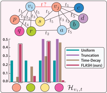
Static heuristics like uniform sampling [Rossi et al., 2020], truncation [Cong et al., 2023] or hybrid approaches [Luo and Li, 2024] are appealing due to their simplicity, but they treat all interactions as equally informative or rely solely on recency. This ignores the fact that some neighbors may be more relevant than others due to their position in the graph or their interaction patterns. Moreover, the optimal sampled neighborhood may vary across time, nodes, and tasks, making fixed strategies fundamentally limited. These shortcomings are further amplified in heterogeneous or rapidly evolving graphs, where structural context can shift dramatically over time. This motivates the need for a learnable, structure-aware neighborhood selection mechanism that can adaptively prioritize informative past interactions.
To address these limitations, we propose FLASH - Flexible Learning of Adaptive Selection from History for Temporal Graph Neural Networks, a learnable and graphadaptive neighborhood selection mechanism for TGNNs. FLASH replaces static heuristics with a data-driven approach that learns to prioritize historically informative neighbors based on their structural and temporal context. Crucially, because the true importance of neighbors is not known a priori, our method is trained using a self-supervised ranking objective that encourages selecting neighbors most predictive of future interactions. FLASH is lightweight, general-purpose, and integrates seamlessly into a wide range of existing TGNN architectures, including TGNNs with non-differentiable feature extractors [Yu et al., 2023; Tian et al., 2023]. This allows it to improve predictive performance without requiring architectural changes. Our key contributions are as follows:
- We propose FLASH, a novel graph-adaptive, learnable neighborhood selection mechanism that seamlessly integrates with any TGNN.
- We design a self-supervised training objective based on ranking loss, enabling our method to learn informative neighbor selection without access to ground-truth labels.
- We provide a theoretical analysis showing that FLASH is provably more expressive than the common heuristics of recent neighbors selection and uniform sampling.
- We conduct extensive experiments across multiple dynamic graph benchmarks, demonstrating consistent performance gains across diverse TGNN backbones compared to common neighbor sampling baselines.
2 RelatedWork
Neighborhood selection in static graphs Existing sampling techniques for large static graphs often rely on substructure sampling (e.g., nodes or edges), as employed by GraphSAGE [Hamilton et al., 2017] and FastGCN [Chen et al., 2018], or utilize random walks, as in PinSage [Ying et al., 2018]. Other methods, such as GraphSAINT [Zeng et al., 2020] and Cluster-GCN [Chiang et al., 2019], are specifically designed to facilitate efficient training on large graphs. However, these approaches typically do not address inference or the temporal nature of dynamic graphs. In many TGNNs, uniform sampling can be viewed as dynamic extension of GraphSAGE-like methods, in which each neighbor in the historical neighborhood is sampled with equal probability. On the other hand, truncation sampling retains only the most recent neighbors, and its stochastic variant of timeweighting, reduces the sampling probability of older neighbors over time, effectively treating recency as a measure of importance. This parallels importance sampling in static graphs (e.g., FastGCN), where recent interactions are explicitly prioritized. However, our experiments show that recency alone is insufficient to capture the complexities of temporal interactions. Instead, incorporating node-specific contextual information at each interaction point, as done by FLASH, proves crucial for achieving robust and accurate performance in dynamic graph settings.
Learning from Large Historical Neighborhoods Learning from large historical neighborhoods in dynamic graphs poses significant challenges in computational cost and capturing long-term dependencies. To address the latter, the patching technique introduced in [Yu et al., 2023], adopted in other recent studies [Tian et al., 2023; Ding et al., 2025]. The method splits the historical neighborhood into chronological patches, each linearly projected into a single representative vector. Since historical neighbors must be encoded (e.g., via co-occurrence encoding [Yu et al., 2023]), neighborhood selection precedes it to reduce computational overhead. Thus, as proposed by [Yu et al., 2023] for DYGFORMER, patching is a complementary strategy for processing large historical neighborhoods, in future link prediction tasks.
Weighing and Selection Mechanisms. Some approaches, such as TGAT [Xu et al., 2020], employ attention mechanisms to weight neighbors, but only after the neighborhood has been sampled. Other works use reinforcement learning [Wang et al., 2022] to learn selection strategies, but they require task-specific reward design and extensive training. Methods based on hard negative mining or curriculum sampling [Younesian et al., 2024] share our motivation of identifying informative samples, but are not tailored for selfsupervised learning and are not readily applicable to TGNNs. In contrast, FLASH learns to sample informative neighbors in a self-supervised, fully differentiable manner.
3 Background
Continuous Time Dynamic Graph (CTDG) is represented as a sequence of time-stamped events G = {(x1, t1), (x2, t2) · · · } where t1 ≤ t2 ≤ · · · . Each event (xi, ti) represents an action on the graph that occurred at time ti. Each such action can be either node addition, node removal, edge addition, or edge removal. We denote Gt = (Vt, Et) the snapshot of CTDG at time t, which is the graph received by applying all the events in G that occurred until time t, where G0 = (∅,∅). We denote FV : V × R+ → RdV and FE : E × R+ → RdE as the functions that map a node or an edge to their features, at a specific point in time. For a given node v and timestamp t, we denote the historic neighborhood Hv,t as the set of all nodes that interacted with v before time t:
Certain TGNNs allow the same node u to appear multiple times in Hv,t, where each occurrence of u is associated with a distinct timestamp that records the time v and u interacted. TGNNs construct node representations by sampling a subset Sv,t(k) ⊆ Hv,t of k historical neighbors. Existing approaches employ various static selection strategies:
where ru is the rank of u with respect to the sequence of sorted neighbors from Hv,t in a decreasing order by their timestamp. Some TGNNs [Rossi et al., 2020] allow sampling beyond the 1-hop historical neighborhood, either by allowing the sampling technique to sample farther nodes in advance or by applying the sampling technique recursively, i.e., sampling from the neighborhood of the sampled neighbors.
Given the sampled neighborhood Sv,t(k), the representation of node v at time t is computed as:
where ψ(·) is a parametric function of the TGNN that maps node to vector based on its sampled neighborhood.
For the task of future link prediction, given a pair of nodes (vi, vj) and their appropriate representations ztvi and ztvj at time t, a TGNN assigns a probability to the existence of a future edge between them using a learnable MERGE function:
To train and evaluate TGNNs for future link prediction, the common approach is to split the entire sequence of interactions into two consecutive non-overlapping segments: a training prefix and an evaluation suffix. All interactions within the training prefix serve as positive examples, indicating node pairs that do form an edge at a specific time. For negative examples, random node pairs are sampled. The TGNN parameters are then updated by minimizing a binary classification loss (e.g., cross-entropy) that distinguishes positive from negative edges:
where yt ij is 1 for observed edges in the training prefix and 0 otherwise. Once trained, the TGNN can be used to predict edges in the evaluation suffix by computing the probability p(vi, vj | t) for new future node pairs.
3.1 Theoretical analysis of Heuristic Neighborhood Samplings
The lack of flexibility in common neighborhood sampling techniques, such as k recent selection (truncation) or uniform sampling, hinder the performance of TGNNs. Specifically, we show that there exist dynamic graphs such that any TGNN relying on these common heuristics cannot learn from them (i.e., it cannot overfit on this graph).
Theorem 1. For any k there exists a dynamic graph on which a TGNN that applies k recent neighbors sampling cannot learn.
Theorem 2. For any k, there exists a dynamic graph on which a TGNN that applies uniform sampling of k historical neighbors cannot learn.
To prove Theorem 1, we find a graph that the k + 1 recent neighbor is required to learn the dynamic behavior of the graph. To prove Theorem 2, we find a dynamic graph that requires consistently selecting the same recent neighbor to learn its dynamic behavior. We provide the full proofs and assumptions for Theorem 1 and Theorem 2 in Appendix D.
Implication. These common sampling heuristics discard potentially crucial historical interactions, limiting the performance of TGNNs and reduce their expressive power. We aim to develop a learnable and adaptive sampling technique that not only generalizes these heuristics but also enables TGNNs to become more expressive.
4 Method
In the previous section, we showed that current neighborhood sampling strategies do not fully account for the graph structure and its features, preventing TGNNs from capturing even simple evolving dynamics. Another limitation of these sampling heuristics stems from the fact that different TGNNs learn temporal dynamics in distinct ways due to their diverse designs. For example, TGN [Rossi et al., 2020] uses memory states, whereas DyGFormer [Yu et al., 2023] employs a Transformer-based architecture [Vaswani et al., 2017] and jointly processes Svi, t and Svj, t. Thus, enforcing the same fixed neighborhood sampling scheme across various TGNNs may undermine their performance. A learnable sampling strategy can adapt not only to the structure of the dynamic graph but also to the way each TGNN architecture exploits temporal signals.
4.1 Desiderata for Adaptive Neighborhood Sampling in TGNNs
We propose an adaptive neighborhood sampling mechanism that satisfies the following desiderata:
- Adapt to CTDG Dynamics: We seek a mechanism SAMPLE(·) that accounts for node and edge attributes as well as their timestamps, i.e., the learnable parameters θ should be informed by the CTDG's interaction patterns. Formally, for a node v with historical neighborhood Hv,t and a candidate interaction partner v′ ,
where |Sv,t| = k.
- Generalize Existing Heuristics: SAMPLE(·) should subsume commonly used heuristics (e.g., truncation, uniform sampling) as special cases via appropriate choices of θ.
- Seamless Integration with TGNNs: Since TGNN backbones encode temporal dynamics differently (e.g., memory modules, attention), the relevance of sampled neighbors may depend on the backbone. Accordingly, the TGNN should inform the sampling procedure and the learning of θ. Moreover, the mechanism should integrate seamlessly with a broad range of TGNNs, including models with non-differentiable feature extractors.
- Self-Supervised Learning of Neighbor Importance: Because ground-truth neighbor "importance" is unavailable, the mechanism should be learnable in a selfsupervised manner that rewards neighbor subsets conducive to accurate link prediction.
4.2 FLASH
To predict a future link (vi, vj) at time t, we learn how informative each historical neighbor u ∈ Hvi,t is for this prediction. Concretely, SAMPLE(·; θ) assigns a score to each historical neighbor and selects the k neighbors with the highest score.
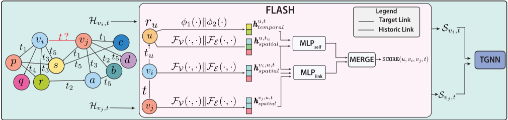
Learning the scoring function. We first construct an informative representation for each historical neighbor that captures both structural (interaction context) and temporal (time-dependent) information (D1). For a neighbor u ∈ Hvi,t, let tu denote the time at which u and vi interacted, and let ru denote the rank of u when sorting Hvi,t in decreasing order of interaction time. We define:
where ϕ1(·) and ϕ2(·) are Time2Vec representations kazemi2019time2vec, FV maps nodes and timestamps to their corresponding features, FE maps edges and timestamps to their corresponding features (as defined in Section 3), M(·) denotes learnable node features, and ∥ denotes concatenation. Following the standard TGNN pipeline and prior work deng2024taser, we project the neighbor and link representations to a common dimensionality using MLPs, and then combine them via a MERGE operator:
where MERGE is an MLP with a single hidden layer, as suggested for combining source-destination information yu2023towards,tian2023freedyg. SCOREu,vi,vj,t measures the utility of neighbor u for predicting the link (vi, vj) at time t, where larger values indicate higher importance. FLASH then selects the k neighbors with the highest scores. Figure 2 provides a detailed schematic of FLASH.
Training FLASH. For each node pair (vi, vj) at time t, let yt ij ∈ {0, 1} indicate whether (vi, vj) is a positive (observed) edge (yt ij = 1) or a negative (unobserved) edge (yt ij = 0). Let a TGNN compute edge probabilities using the subsets selected by FLASH, (Svi,vj,t, Svj,vi,t), and using uniformly sampled subsets (S uni vi ,t , S uni vj,t ). We define the probability difference:
Let svi , svj denote the average FLASH scores over nodes in Svi,vj,t and Svj,vi,t, respectively, and let suni vi , suni vj denote the corresponding averages over S uni vi,t and S uni vj,t . For positive edges, we prefer ∆tij > 0 (our subsets increase the predicted probability), while for negative edges we prefer ∆tij < 0 (our subsets decrease it). We enforce this preference using a pairwise RankNet burges2005learning logistic loss:
Minimizing Ltij encourages the score averages to move in the direction consistent with yt ij without requiring any ground-truth importance supervision (D3). When the condition in Equation (14) holds, the neighborhoods selected by FLASH improve over uniform sampling, and the loss encourages higher scores for selected neighbors over the uniformly sampled neighbors. Otherwise, uniform sampling performs better and the loss correspondingly increases the scores of uniformly sampled neighbors relative to those selected by FLASH. We train FLASH jointly with a given TGNN by optimizing the sum of Equation (14) and Equation (6). Gradients from Equation (6) update only the TGNN parameters, while for Equation (14) we stop gradients through ∆tij so that updates flow only to FLASH parameters (D4). To ensure constant runtime, FLASH first applies a recent-neighbors finder deng2024taser to restrict the candidate set to a fixed size. It then computes scores only within this reduced neighborhood rather than over the full historical neighborhood. In Appendix G, we provide a throughout analysis of FLASH and TASER.
| Method ↓ / Dataset → | WIKIPEDIA AP ↑ | REDDIT AP ↑ | MOOC AP ↑ | LASTFM AP ↑ | SOCIAL EVO. AP ↑ | ENRON AP ↑ | UCI AP ↑ |
|---|---|---|---|---|---|---|---|
| TGAT + Trunc. | 94.05±0.06 | 93.63±0.16 | 79.69±0.24 | 65.64±0.34 | 85.36±0.25 | 72.91±0.58 | 79.74±0.37 |
| TGAT + Uni. | 62.60±0.36 | 87.94±0.03 | 60.03±0.11 | 50.66±0.11 | 53.22±0.79 | 51.34±0.32 | 60.42±0.22 |
| TGAT + NLB | 91.49±0.25 | 92.78±0.11 | 77.37±0.17 | 65.64±0.34 | 83.19±0.07 | 70.69±0.93 | 77.80±1.25 |
| TGAT + TASER | 67.78±0.99 | 89.14±0.59 | 67.10±0.56 | 52.28±0.52 | 70.40±0.45 | 60.55±0.91 | 70.62±0.33 |
| TGAT + FLASH | 94.67±0.38 | 95.92±0.13 | 80.24±0.54 | 74.94±1.49 | 92.17±0.25 | 79.04±0.94 | 87.84±0.12 |
| TGN + Trunc. | 98.55±0.05 | 98.61±0.03 | 90.13±0.64 | 82.62±2.09 | 91.63±0.51 | 86.51±2.29 | 93.34±0.25 |
| TGN + Uni. | 98.49±0.08 | 98.59±0.01 | 83.08±1.11 | 67.60±5.66 | 65.52±6.06 | 85.47±2.00 | 93.34±0.25 |
| TGN + NLB | 98.31±0.09 | 98.61±0.04 | 89.81±0.60 | 80.45±1.94 | 91.19±0.38 | 86.51±2.29 | 92.91±0.43 |
| TGN + TASER | 98.15±0.07 | 98.63±0.04 | 90.57±1.02 | 75.58±4.07 | 92.24±0.62 | 86.87±0.081 | 89.86±2.61 |
| TGN + FLASH | 98.73±0.06 | 99.06±0.03 | 91.19±0.51 | 90.54±0.62 | 93.43±0.11 | 89.90±0.76 | 95.17±0.16 |
| GRAPHMIXER + Trunc. | 96.23±0.24 | 95.17±0.03 | 80.71±0.11 | 72.98±0.07 | 87.09±0.12 | 81.63±0.47 | 93.14±0.44 |
| GRAPHMIXER + Uni. | 77.06±0.16 | 89.80±0.05 | 64.75±0.39 | 63.96±0.09 | 55.69±0.12 | 55.65±3.04 | 71.27±2.79 |
| GRAPHMIXER + NLB | 95.09±0.12 | 95.17±0.03 | 78.61±0.09 | 72.98±0.07 | 85.66±0.09 | 81.01±0.30 | 92.51±0.60 |
| GRAPHMIXER + TASER | 93.27±1.43 | 94.78±0.17 | 78.97±0.66 | 72.24±0.93 | 87.57±2.53 | 77.90±0.48 | 88.59±1.10 |
| GRAPHMIXER + FLASH | 97.51±0.25 | 96.62±0.11 | 80.85±0.52 | 82.68±0.74 | 92.84±0.11 | 85.74±0.70 | 93.21±0.61 |
| DYGFORMER + Trunc. | 96.91±0.05 | 95.15±0.07 | 82.47±0.07 | 74.81±0.09 | 85.73±0.06 | 82.35±0.66 | 89.61±0.22 |
| DYGFORMER + Uni. | 96.87±0.07 | 95.15±0.07 | 82.47±0.07 | 74.81±0.09 | 85.71±0.06 | 82.35±0.66 | 89.61±0.22 |
| DYGFORMER + NLB | 96.74±0.07 | 95.03±0.09 | 81.09±0.05 | 74.52±0.18 | 85.40±0.10 | 81.86±0.45 | 89.12±0.19 |
| DYGFORMER + TASER | 95.47±0.32 | 93.83±0.33 | 81.56±0.67 | 72.72±1.73 | 90.09±0.11 | 81.74±0.64 | 88.15±0.59 |
| DYGFORMER + FLASH | 98.17±0.04 | 98.11±0.02 | 82.96±0.42 | 86.09±0.13 | 92.41±0.11 | 88.70±0.17 | 92.96±0.16 |
| FREEDYG + Trunc. | 98.35±0.01 | 97.53±0.02 | 85.02±0.02 | 80.19±0.04 | 90.88±0.05 | 88.77±0.20 | 95.21±0.33 |
| FREEDYG + Uni. FREEDYG + NLB | 98.33±0.02 98.33±0.01 | 95.98±0.03 97.59±0.02 | 67.52±0.18 83.56±0.12 | 67.72±0.10 80.02±0.09 | 89.16±0.03 90.40±0.05 | 88.46±0.08 88.77±0.20 | 95.21±0.33 95.17±0.26 |
| FREEDYG + TASER | 97.94±0.35 | 97.11±0.30 | 76.97±3.87 | 78.54±1.90 | 90.84±1.09 | 87.24±1.47 | 93.15±1.46 |
| 98.94±0.04 | |||||||
| FREEDYG + FLASH | 98.72±0.02 | 85.69±0.27 | 88.46±0.07 | 93.62±0.05 | 91.31±0.01 | 95.86±0.16 |
4.3 Theoretical Analysis of FLASH
The components of FLASH adapt to the evolution of the dynamic graph over time and to the interactions being predicted, by incorporating both spatiotemporal features and potentially interacting nodes when constructing each sampled neighborhood. We show that FLASH can replicate both k-recent neighbor selection and uniform sampling. Furthermore, we show that the graphs used in the proofs of Theorem 1 and Theorem 2 can be learned by a TGNN that utilizes FLASH. Therefore:
Theorem 3. FLASH is more expressive than k-recent neighbor selection and uniform sampling.
We provide the full proof of Theorem 3 in Appendix D.
5 Experiments
We evaluate FLASH across multiple dynamic graph benchmarks and compare it with recent state-of-the-art baselines.
Section 5.1 presents our key empirical findings, and Section 5.2 provides additional ablation studies. Additional results are reported in Appendix C. Our experiments aim to answer the following research questions:
- (RQ1) How does our proposed strategy compare to established sampling baselines in predictive accuracy?
- (RQ2) Does our method generalize across varying graph sizes, sparsity levels, and temporal granularities?
- (RQ3) What is the computational overhead of our approach relative to existing methods?
Experimental Setup. We test our method on five common TGNNs: TGAT [Xu et al., 2020], TGN [Rossi et al., 2020], GRAPHMIXER [Cong et al., 2023], DYGFORMER [Yu et al., 2023], and FREEDYG [Tian et al., 2023]. Detailed descriptions of each model are provided in Appendix B. Each model is trained with four neighbor sampling strategies: Truncation [Cong et al., 2023; Yu et al., 2023], Uniform [Rossi et al., 2020], No-Look-Back (NLB) [Luo and Li, 2024], TASER with the recent-neighbors finder and a linear predictor [Deng et al., 2024], and our proposed method. Following standard practice, we use a chronological 70%-15%-15% train-validation-test split. Additional parameters regarding the training scheme and implementation-specific details are provided in Appendix E.
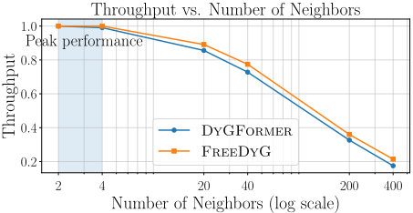
Importance of Small Neighborhoods As discussed in Section 1, processing large neighborhoods is computationally prohibitive in both time and space. Figure 4 reports the throughput of state-of-the-art TGNNs for varying neighborhood sizes. The results show that increasing the neighborhood processed in parallel substantially degrades model throughput. Consequently, TGNNs should employ small neighborhoods (2-4) to achieve peak runtime performance. Accordingly, we evaluate neighborhood selection strategies under a small neighborhood budget (2-4) to determine which strategy is optimal for future link prediction while sustaining peak throughput in TGNNs.
| Method ↓ / Dataset → | WIKIPEDIA AP ↑ | REDDIT AP ↑ | MOOC AP ↑ | LASTFM AP ↑ | SOCIAL EVO. AP ↑ | ENRON AP ↑ | UCI AP ↑ |
|---|---|---|---|---|---|---|---|
| TGAT + Trunc. TGAT + Uni. | 94.26±0.09 | 90.82±0.18 | 78.12±0.18 | 72.35±0.42 | 82.73±0.29 53.06±0.40 | 70.25±1.30 51.63±0.72 | 80.95±0.29 |
| 62.77±0.43 | 82.85±0.13 | 58.38±0.14 | 50.75±0.07 | 59.65±0.36 | |||
| TGAT + NLB. | 91.46±0.24 | 89.70±0.15 | 75.42±0.22 | 72.35±0.42 | 80.66±0.12 | 68.77±1.03 | 78.47±0.68 |
| TGAT + TASER | 67.62±1.08 | 84.51±0.75 | 63.60±0.52 | 53.53±0.85 | 67.22±0.59 | 58.46±1.38 | 64.94±0.90 |
| TGAT+FLASH | 94.70±0.35 | 94.24±0.10 | 78.85±0.61 | 79.56±1.57 | 90.23±0.25 | 76.70±1.13 | 87.77±0.17 |
| TGN + Trunc. | 97.84±0.05 | 97.28±0.08 | 90.02±1.30 | 87.23±1.18 | 89.08±1.42 | 79.66±2.23 | 89.36±0.52 |
| TGN + Uni. | 97.82±0.12 | 97.13±0.15 | 82.47±0.41 | 76.10±6.58 | 57.15±0.35 | 77.91±2.34 | 89.36±0.52 |
| TGN + NLB. | 97.61±0.08 | 97.23±0.09 | 89.19±0.48 | 85.79±2.00 | 86.51±2.51 | 79.66±2.23 | 88.34±0.52 |
| TGN + TASER | 97.39±0.17 | 97.33±0.12 | 89.90±1.18 | 81.97±3.73 | 90.31±1.50 | 78.99±2.56 | 85.28±1.22 |
| TGN+FLASH | 98.08±0.12 95.80±0.24 | 98.24±0.07 92.21±0.07 | 90.50±0.61 79.38±0.18 | 92.04±0.40 79.52±0.11 | 92.06±0.48 | 82.95±1.02 | 92.40±0.27 |
| GraphMixer + Trunc. GraphMixer + Uni. | 78.72±0.12 | 84.29±0.10 | 65.91±0.30 | 73.74±0.07 | 84.83±0.14 51.13±0.15 | 76.17±0.43 52.46±3.33 | 91.60±0.19 71.69±1.43 |
| GraphMixer + NLB | 94.34±0.10 | 92.21±0.07 | 76.89±0.10 | 79.52±0.11 | 83.09±0.08 | 74.99±0.34 | 90.89±0.23 |
| GraphMixer | 92.42±1.54 | 91.25±0.30 | 79.43±1.02 | 85.10±2.73 | 70.70±0.44 | 86.78±1.76 | |
| +TASER | 76.99±0.59 | 90.74±0.11 | |||||
| GraphMixer + FLASH | 97.06±0.29 | 94.77±0.21 | 79.44±0.55 | 86.70±0.74 | 80.61±1.41 | 91.66±0.24 | |
| DyGFormer + Trunc. DyGFormer + Uni. | 97.02±0.07 97.01±0.06 | 93.40±0.08 93.40±0.08 | 81.27±0.09 81.27±0.09 | 79.97±0.11 79.86±0.12 | 82.86±0.07 82.80±0.07 | 80.46±0.91 80.46±0.91 | 89.99±0.18 89.81±0.16 |
| DyGFormer + | 96.86±0.08 | 93.27±0.09 | 80.09±0.38 | 89.52±0.22 | |||
| NLB | 79.62±0.11 | 79.66±0.23 | 82.68±0.10 | ||||
| DyGFormer + TASER | 95.70±0.26 | 91.05±0.51 | 80.37±0.65 | 77.93±1.60 | 88.20±0.25 | 79.28±1.20 | 84.98±0.58 |
| DyGFormer + FLASH | 97.91±0.04 | 97.36±0.04 | 81.42±0.51 | 88.55±0.15 | 90.56±0.28 | 84.88±0.66 | 92.73±0.15 |
| FreeDyG + Trunc. | 98.03±0.03 | 96.34±0.04 | 84.04±0.06 | 85.09±0.07 | 89.06±0.09 | 84.59±0.33 | 93.98±0.15 |
| FreeDyG + Uni. FreeDyG + NLB. | 98.01±0.02 97.99±0.01 | 93.86±0.04 96.34±0.04 | 68.53±0.24 82.13±0.10 | 76.41±0.09 84.98±0.13 | 86.92±0.09 88.38±0.17 | 83.96±0.21 84.59±0.33 | 93.98±0.15 93.81±0.16 |
| FreeDyG +TASER | 97.67±0.34 | 95.63±0.38 | 74.93±4.60 | 84.07±1.25 | 88.87±1.17 | 81.31±2.04 | 92.02±1.32 |
| FreeDyG + FLASH | 98.59±0.03 | 98.21±0.04 | 84.38±0.25 | 90.73±0.09 | 91.53±0.63 | 87.13±0.62 | 94.60±0.13 |
5.1 Results
Evaluation with DyGLib. We use the WIKIPEDIA, REDDIT, MOOC, LASTFM, ENRON, SOCIAL EVO., and UCI datasets from the DyGLib benchmark [Yu et al., 2023]. DyGLib includes datasets spanning a wide range of graph sizes, with some containing over a million edges (RQ2). Full dataset statistics are provided in Appendix A. We evaluate future edge prediction (Equation (6)) under two settings: (1) transductive, where all nodes appear during training, and (2)
| ϕ2 ϕ1MMLPlink WIKIPEDIA | ENRON UCI | ||
| ✗ ✓ | ✓ | ✓ ✓ | 98.73±0.07 89.63±0.72 95.08±0.19 98.20±0.06 89.50±0.74 95.08±0.33 98.58±0.06 86.45±1.25 93.27±0.61 98.54±0.09 87.38±0.81 93.06±0.60 |
| ✗ ✗ | ✓ | ||
| ✓ ✓ | ✗ | ✓ | |
| ✓ ✓ | ✓ | ✗ | |
| ✓ ✓ | ✓ | ✓ | 98.73±0.06 89.90±0.76 95.17±0.16 |
inductive, where test nodes are unseen during training. Tables 1 and 2 report results across models and methods. Overall, FLASH consistently outperforms previously suggested neighborhood selection strategies, both in the transductive setting and the inductive setting (RQ1). For example, on SOCIAL EVO., FLASH achieves a ∼8% relative improvement over truncation for TGAT, and on LASTFM, a ∼15% relative improvement for FREEDYG, demonstrating strong effectiveness even for computationally expensive models.
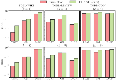
Evaluation with TGB. We evaluate FLASH on the TGB benchmark [Huang et al., 2023] using TGBL-WIKI, TGBLREVIEW, and TGBL-COIN. In contrast to DyGLib, TGB samples multiple random negative edges for each positive edge and is evaluated using Mean Reciprocal Rank (MRR). From Figure 3, FLASH yields performance that is consistently on par with or better than baselines across TGNNs and neighborhood sizes. Notably, on TGBL-REVIEW, our method improves performance by ∼2.67× for GRAPHMIXER when k = 4, highlighting robustness across diverse dynamic graph scenarios (RQ2).
5.2 Ablation Study
FLASH Design Choices. We ablate key components of FLASH, namely the historical position embedding ϕ2, temporal embedding ϕ1, learnable node embedding M, and the link-awareness module MLPlink in Equation (12), to assess the contribution of temporal, structural, and interaction context for future edge prediction (RQ2). Table 3 shows that the positional embedding ϕ2 is particularly important on ENRON and UCI, indicating that relying solely on temporal information is suboptimal. The interaction context module, MLPlink, is consistently beneficial across all datasets, providing reliable performance improvements.
Computational Overhead. Table 4 reports a throughput comparison for FLASH, measured as the number of processed edges per second, against the baselines (RQ3). For a fair comparison, both TASER and FLASH employ the same neighbor finder, which constrains their neighborhoods to an identical size, this benefits both methods relative to uniform sampling. Because all experiments use a unified batch size, model latency is inversely proportional to throughput. Appendix F further provides a time-complexity analysis of FLASH and the baselines.
| Model | Uniform | NLB | TASER | FLASH |
|---|---|---|---|---|
| TGAT | 51% | 44% | 59% | 75% |
| TGN | 67% | 80% | 82% | 82% |
| GRAPHMIXER | 42% | 40% | 59% | 64% |
| DYGFORMER | 97% | 87% | 86% | 94% |
| FREEDYG | 84% | 85% | 91% | 92% |
6 Conclusion
In this work, we introduce FLASH, a flexible, end-to-end learnable neighborhood selection framework for dynamic graph learning. FLASH factorizes the neighbor scoring function into spatial and temporal components, ensuring that neighbor importance reflects both topological structure and temporal context. Our training objective couples the learned scores with downstream predictive performance, enabling effective optimization of the selection policy even when ground-truth importance scores are unavailable and TGNN operations are non-differentiable. This design allows FLASH to integrate seamlessly with a broad range of TGNN architectures, providing an efficient mechanism for selecting the most relevant historical neighbors. We further evaluate FLASH across multiple dynamic graph benchmarks and show that it matches or outperforms the considered baselines.
Contribution Statement
O.F. contributed to the design of the method, implementation, experiments, figure/plot design, and manuscript writing. K.S.I.M. contributed to the design of the method, figure/plot design, and manuscript writing. C.B.S. contributed to manuscript writing. C.B. and M.E. contributed to manuscript writing and equally supervised the work.
@inproceedings{ijcai2026p476,
  title     = {FLASH: Flexible Learning of Adaptive Sampling from History in Temporal Graph Neural Networks},
  author    = {Feldman, Or and Mantri, Krishna Sri Ipsit and Schönlieb, Carola-Bibiane and Baskin, Chaim and Eliasof, Moshe},
  booktitle = {Proceedings of the Thirty-Fifth International Joint Conference on
               Artificial Intelligence, {IJCAI-26}},
  publisher = {International Joint Conferences on Artificial Intelligence Organization},
  editor    = {Diego Calvanese},
  pages     = {4278--4285},
  year      = {2026},
  month     = {8},
  note      = {Main Track},
  doi       = {10.24963/ijcai.2026/476},
  url       = {https://doi.org/10.24963/ijcai.2026/476},
}
TY - CPAPER TI - FLASH: Flexible Learning of Adaptive Sampling from History in Temporal Graph Neural Networks AU - Feldman, Or AU - Mantri, Krishna Sri Ipsit AU - Schönlieb, Carola-Bibiane AU - Baskin, Chaim AU - Eliasof, Moshe T2 - Proceedings of the Thirty-Fifth International Joint Conference on Artificial Intelligence, IJCAI-26 PB - International Joint Conferences on Artificial Intelligence Organization PY - 2026 SP - 4278 EP - 4285 DO - 10.24963/ijcai.2026/476 UR - https://doi.org/10.24963/ijcai.2026/476 ER -Copied
Machine-readable versions of this paper, for tools and AI agents:





