
Efficient Algorithms for Influence Maximization in General Models and Observed Cascades
Proceedings of the Thirty-Fifth International Joint Conference on Artificial Intelligence. Main Track. Pages 348-356.
https://doi.org/10.24963/ijcai.2026/40
Keywords
- Agent-based and Multi-agent Systems: Resource allocation
- Search: Combinatorial search and optimisation
- Data Mining: Mining graphs
Abstract
We study influence maximization in general stochastic models, the observed cascades model, and the independent cascade (IC) model. For general stochastic models with only black-box sample access, we introduce a low-adaptivity optimization framework that improves sample complexity and running time over the prior work and is instrumental to all our results. We further introduce an adaptive algorithm guided by empirical variance, avoiding pessimistic worst-case bounds. Combining our optimization framework with sketching, we obtain the first algorithm with provable guarantees and nearly-linear running time for influence maximization on observed cascades, optimal up to logarithmic factors. For IC, we prove a novel tail bound replacing a factor n with ? (the number of diffusion steps) in sample complexity, improving over prior work when ? is small, as is common due to small-world phenomena. Experiments confirm substantial speedups while maintaining solution quality.
- [Balkanski and Singer, 2018] Eric Balkanski and Yaron Singer. The adaptive complexity of maximizing a submod- ular function. In STOC, pages 1138-1151. ACM, 2018.
- [Balkanski et al., 2022] Eric Balkanski, Aviad Rubinstein, and Yaron Singer. The limitations of optimization from samples. J. ACM, 69(3):21:1-21:33, 2022.
- [Borgs et al., 2014] Christian Borgs, Michael Brautbar, Jen- nifer T. Chayes, and Brendan Lucier. Maximizing social influence in nearly optimal time. In SODA, pages 946- 957. SIAM, 2014.
- [Bringmann and Friedrich, 2013] Karl Bringmann and To- bias Friedrich. Exact and efficient generation of geometric random variates and random graphs. In ICALP (1), vol- ume 7965 of Lecture Notes in Computer Science, pages 267-278. Springer, 2013.
- [Chen et al., 2010] Wei Chen, Chi Wang, and Yajun Wang. Scalable influence maximization for prevalent viral mar- keting in large-scale social networks. In KDD, pages 1029-1038. ACM, 2010.
- [Chen et al., 2012] Wei Chen, Wei Lu, and Ning Zhang. Time-critical influence maximization in social networks with time-delayed diffusion process. In AAAI, pages 591- 598. AAAI Press, 2012.
- [Chen et al., 2013] Wei Chen, Laks V. S. Lakshmanan, and Carlos Castillo. Information and Influence Propagation in Social Networks. Synthesis Lectures on Data Manage- ment. Morgan & Claypool Publishers, 2013.
- [Chen et al., 2021a] Wei Chen, Xiaoming Sun, Jialin Zhang, and Zhijie Zhang. Network inference and influence maxi- mization from samples. In ICML, volume 139 of Proceed- ings of Machine Learning Research, pages 1707-1716. PMLR, 2021.
- [Chen et al., 2021b] Yixin Chen, Tonmoy Dey, and Alan Kuhnle. Best of both worlds: Practical and theoretically optimal submodular maximization in parallel. In NeurIPS, pages 25528-25539, 2021.
- [Cohen and Kaplan, 2007] Edith Cohen and Haim Kaplan. Summarizing data using bottom-k sketches. In PODC, pages 225-234. ACM, 2007.
- [Cohen et al., 2014a] Edith Cohen, Daniel Delling, Thomas Pajor, and Renato F. Werneck. Sketch-based influence maximization and computation: Scaling up with guaran- tees. CoRR, abs/1408.6282, 2014.
- [Cohen et al., 2014b] Edith Cohen, Daniel Delling, Thomas Pajor, and Renato F. Werneck. Timed influence: Compu- tation and maximization. CoRR, abs/1410.6976, 2014.
- [Cohen, 1997] Edith Cohen. Size-estimation framework with applications to transitive closure and reachability. J. Comput. Syst. Sci., 55(3):441-453, 1997.
- [Du et al., 2013] Nan Du, Le Song, Manuel Gomez- Rodriguez, and Hongyuan Zha. Scalable influence esti- mation in continuous-time diffusion networks. In NIPS, pages 3147-3155, 2013.
- [Gomez-Rodriguez et al., 2011] Manuel Gomez-Rodriguez, David Balduzzi, and Bernhard Schölkopf. Uncovering the temporal dynamics of diffusion networks. In ICML, pages 561-568. Omnipress, 2011.
- [Granovetter, 1978] Mark Granovetter. Threshold models of collective behavior. American journal of sociology, 83(6):1420-1443, 1978.
- [Guo et al., 2022] Qintian Guo, Sibo Wang, Zhewei Wei, Wenqing Lin, and Jing Tang. Influence maximization re- visited: Efficient sampling with bound tightened. ACM Trans. Database Syst., 47(3):12:1-12:45, 2022.
- [Huang et al., 2017] Keke Huang, Sibo Wang, Glenn S. Bevilacqua, Xiaokui Xiao, and Laks V. S. Lakshmanan. Revisiting the stop-and-stare algorithms for influence maximization. Proc. VLDB Endow., 10(9):913-924, 2017.
- [Kempe et al., 2015] David Kempe, Jon M. Kleinberg, and Éva Tardos. Maximizing the spread of influence through a social network. Theory Comput., 11:105-147, 2015.
- [Kolli and Narayanaswamy, 2019] Naimisha Kolli and Bal- akrishnan Narayanaswamy. Influence maximization from cascade information traces in complex networks in the ab- sence of network structure. IEEE Trans. Comput. Soc. Syst., 6(6):1147-1155, 2019.
- [Leskovec and Krevl, 2014] Jure Leskovec and Andrej Krevl. SNAP Datasets: Stanford large network dataset collection. http://snap.stanford.edu/data, June 2014. Link
- [Leskovec et al., 2007a] Jure Leskovec, Andreas Krause, Carlos Guestrin, Christos Faloutsos, Jeanne M. Van- Briesen, and Natalie S. Glance. Cost-effective outbreak detection in networks. In KDD, pages 420-429. ACM, 2007.
- [Leskovec et al., 2007b] Jure Leskovec, Mary McGlohon, Christos Faloutsos, Natalie S. Glance, and Matthew Hurst. Patterns of cascading behavior in large blog graphs. In SDM, pages 551-556. SIAM, 2007.
- [Li et al., 2023] Yandi Li, Haobo Gao, Yunxuan Gao, Jianx- iong Guo, and Weili Wu. A survey on influence maximiza- tion: From an ml-based combinatorial optimization. ACM Trans. Knowl. Discov. Data, 17(9):133:1-133:50, 2023.
- [Ling et al., 2023] Chen Ling, Junji Jiang, Junxiang Wang, My T. Thai, Lukas Xue, James Song, Meikang Qiu, and Liang Zhao. Deep graph representation learning and optimization for influence maximization. CoRR, abs/2305.02200, 2023.
- [Liu et al., 2012] Bo Liu, Gao Cong, Dong Xu, and Yifeng Zeng. Time constrained influence maximization in social networks. In ICDM, pages 439-448. IEEE Computer So- ciety, 2012.
- [Mirzasoleiman et al., 2015] Baharan Mirzasoleiman, Ash- winkumar Badanidiyuru, Amin Karbasi, Jan Vondrák, and Andreas Krause. Lazier than lazy greedy. In AAAI, pages 1812-1818. AAAI Press, 2015.
- [Mossel and Roch, 2007] Elchanan Mossel and Sébastien Roch. On the submodularity of influence in social net- works. In STOC, pages 128-134. ACM, 2007.
- [Narasimhan et al., 2015] Harikrishna Narasimhan, David C. Parkes, and Yaron Singer. Learnability of influence in networks. In NIPS, pages 3186-3194, 2015.
- [Nemhauser et al., 1978] George L. Nemhauser, Lau- rence A. Wolsey, and Marshall L. Fisher. An analysis of approximations for maximizing submodular set functions -I. Math. Program., 14(1):265-294, 1978.
- [Netrapalli and Sanghavi, 2012] Praneeth Netrapalli and Su- jay Sanghavi. Learning the graph of epidemic cascades. In SIGMETRICS, pages 211-222. ACM, 2012.
- [Nguyen et al., 2016] Hung T. Nguyen, My T. Thai, and Thang N. Dinh. Stop-and-stare: Optimal sampling algo- rithms for viral marketing in billion-scale networks. In SIGMOD Conference, pages 695-710. ACM, 2016.
- [Nguyen et al., 2018] Hung T. Nguyen, Thang N. Dinh, and My T. Thai. Revisiting of 'revisiting the stop-and-stare al- gorithms for influence maximization'. In CSoNet, volume 11280 of Lecture Notes in Computer Science, pages 273- 285. Springer, 2018.
- [Pouget-Abadie and Horel, 2015] Jean Pouget-Abadie and Thibaut Horel. Inferring graphs from cascades: A sparse recovery framework. CoRR, abs/1505.05663, 2015.
- [Richardson and Domingos, 2002] Matthew Richardson and Pedro M. Domingos. Mining knowledge-sharing sites for viral marketing. In KDD, pages 61-70. ACM, 2002.
- [Sadeh et al., 2020] Gal Sadeh, Edith Cohen, and Haim Ka- plan. Sample complexity bounds for influence maximiza- tion. In ITCS, volume 151 of LIPIcs, pages 29:1-29:36. Schloss Dagstuhl -Leibniz-Zentrum für Informatik, 2020.
- [Tang et al., 2014] Youze Tang, Xiaokui Xiao, and Yanchen Shi. Influence maximization: near-optimal time complex- ity meets practical efficiency. In SIGMOD Conference, pages 75-86. ACM, 2014.
- [Tang et al., 2015] Youze Tang, Yanchen Shi, and Xiaokui Xiao. Influence maximization in near-linear time: A mar- tingale approach. In SIGMOD Conference, pages 1539- 1554. ACM, 2015.
- [Tang et al., 2018] Jing Tang, Xueyan Tang, Xiaokui Xiao, and Junsong Yuan. Online processing algorithms for influ- ence maximization. In SIGMOD Conference, pages 991- 1005. ACM, 2018.
- [Travers and Milgram, 2006] Jeffrey Travers and Stanley Milgram. An experimental study of the small world prob- lem, pages 130-148. Princeton University Press, Prince- ton, 2006.
- [Vondrák, 2010] Jan Vondrák. A note on concentration of submodular functions. CoRR, abs/1005.2791, 2010.
- [Yao et al., 2022] Shunyu Yao, Neng Fan, and Jie Hu. Mod- eling the spread of infectious diseases through influence maximization. Optim. Lett., 16(5):1563-1586, 2022.
- [Zhang et al., 2024] Shiqi Zhang, Jiachen Sun, Wenqing Lin, Xiaokui Xiao, Yiqian Huang, and Bo Tang. Infor- mation diffusion meets invitation mechanism. In WWW (Companion Volume), pages 383-392. ACM, 2024.
References were extracted automatically from the PDF and may contain errors.
Full text extracted automatically from the PDF; figures, tables and equations may differ. The PDF is the version of record.
1 Introduction
Understanding diffusion processes in networks is a fundamental problem in computer science, biology, sociology, economics, and other fields. Diffusion processes model phenomena such as the spread of news on social media and the outbreak of a disease [Chen et al., 2013; Yao et al., 2022; Leskovec et al., 2007b]. A typical diffusion process starts with an initial set of active nodes, called the seed set, and it proceeds in discrete time steps. In each step, all previously activated nodes remain active and new nodes become active according to an underlying model of diffusion [Kempe et al., 2015]. The influence of a seed set is the number of nodes that are active at the end of the process. A fundamental optimization problem that arises in many applications is to find a seed set of size at most k (the budget) with maximum influence. Notable applications of influence maximization are viral marketing [Richardson and Domingos, 2002] and outbreak detection in networks [Leskovec et al., 2007a]. In viral marketing, the goal is to find an initial seed set of "influencers" to advertise a product and spread its adoption through the network. In outbreak detection, we would like to monitor a network such as a water distribution network using sensors, and the goal is to find the locations of the sensors that will allow us to detect contaminations as quickly as possible.
Starting with the influential work of Kempe et al. [2015], there has been significant interest in designing algorithms for influence maximization that achieve provable approximation guarantees in general settings. As shown by Kempe et al. [2015] and subsequent work [Mossel and Roch, 2007], a very general class of models where provable approximation guarantees are achievable in polynomial time are submodular stochastic diffusion models, where the expected influence is submodular. Submodular models have significant modeling power and wide-ranging applications, which motivates the design of efficient algorithms that scale to large networks. However, despite important developments for the independent cascade (IC) model [Borgs et al., 2014; Guo et al., 2022; Tang et al., 2014] and more general submodular models [Sadeh et al., 2020], it remains challenging to obtain scalable algorithms for models beyond IC. A key bottleneck is the number of adaptive rounds: the classical Greedy algorithm requires k rounds, each evaluating n candidates (where n is the number of nodes and k the budget), with each evaluation potentially requiring expensive sampling or graph traversals. Recent work on low-adaptivity submodular optimization [Balkanski and Singer, 2018; Chen et al., 2021b] shows that far fewer rounds suffice with exact evaluations, but extending this to stochastic settings is non-trivial. In this work, we develop such an extension, combining low-adaptivity optimization with tailored estimation techniques to obtain faster algorithms with provable guarantees.
Beyond stochastic models, practitioners often work directly with observed data when model parameters are unknown or hard to estimate [Narasimhan et al., 2015]. We therefore also consider the observed cascades setting, where diffusion spreads deterministically according to observed data. Here we develop the first algorithm with provable guarantees and nearly-linear running time, which is optimal up to logarithmic factors.
We handle both unrestricted influence and settings with explicit limits on the number of diffusion steps τ . Restricting τ is necessary in time-critical applications [Chen et al., 2012; Cohen et al., 2014b; Du et al., 2013; Liu et al., 2012; Gomez-Rodriguez et al., 2011], e.g., detecting outbreaks early [Leskovec et al., 2007a]. Moreover, due to "smallworld" phenomena, few-step diffusion often approximates unrestricted influence well [Travers and Milgram, 2006].
1.1 Our contributions
We provide new algorithms with theoretical guarantees for influence maximization in general stochastic models, the observed cascades model, and the independent cascade (IC) model. Our main contributions are:
- Low-adaptivity optimization framework: We adapt the low-adaptivity Greedy algorithm of Chen et al. [2021b] to work with stochastic estimates. This is nontrivial: stochastic estimates are not submodular [Kempe et al., 2015; Balkanski et al., 2022], so the original analysis fails. We develop new techniques to handle the estimation error. This framework is instrumental to all our results: it directly improves sample complexity and running time over Sadeh et al. [2020] by a factor of (almost) k, and makes variance-based estimation and sketching viable.
- Empirical variance estimation: Building on our framework, we introduce an adaptive sampling algorithm guided by empirical variance, avoiding pessimistic worst-case variance bounds required by prior work [Sadeh et al., 2020].
- Nearly-linear time for observed cascades: Combining our framework with sketching [Cohen and Kaplan, 2007], we provide the first algorithm with provable guarantees and nearly-linear ˜O(mtot) running time (where mtot is the input size) for observed cascades, improving over the previously best achievable Ω(n · mtot). Prior work [Cohen et al., 2014a] also uses sketching but with a different algorithmic approach (see Section 3.3).
- New concentration bound for IC: We prove a novel tail bound for IC samples, improving sample complexity by replacing a factor n with τ, yielding improved guarantees over Borgs et al. [2014; 2014; 2022] when τ ≪ n.
Together, these contributions yield algorithms with provable guarantees that substantially improve running time, memory, and sample complexity for both restricted and unrestricted influence.
Practical baselines: Highly optimized practical algorithms exist primarily for the IC model [Borgs et al., 2014; Tang et al., 2014; Tang et al., 2015; Nguyen et al., 2016; Guo et al., 2022]. For general stochastic models and observed cascades, the only prior algorithms with theoretical guarantees are variants of Greedy [Sadeh et al., 2020; Cohen et al., 2014a], which we significantly outperform. These settings are important in practice when IC assumptions do not hold or model parameters are unknown.
1.2 RelatedWork
Influence maximization is well-studied with extensive prior work. We focus on efficient algorithms with theoretical guarantees; for heuristic methods, we refer the reader to Li et al. [2023].
General Stochastic Models: Kempe et al. [2015] show that influence maximization generalizes the maximum coverage problem, and thus it is NP-hard to approximate to any factor better than 1-1/e. They also show that the influence function is submodular for the IC and linear threshold (LT) models, and show how to obtain a nearly-optimal 1- 1e -ϵ approximation with high probability by implementing the Greedy algorithm [Nemhauser et al., 1978] using stochastic estimates for the marginal gains obtained from simulations of the model. Even though the running time of their approach is polynomial, it is prohibitive in practice. Kempe et al. [2015] introduce a more general stochastic diffusion model, called the General Threshold model, a vast generalization of the IC, LT, and other diffusion models. Subsequently, Mossel and Roch [2007] show that the influence function is submodular in General Threshold models with submodular activation functions. Sadeh et al. [2020] study sample complexity of influence maximization in general models, including General Threshold models, parameterized by the number of diffusion steps, providing improved sample complexity and running time.
Independent Cascades: Borgs et al. [2014] introduce reverse influence sampling which is specialized to the IC model, but offers significantly improved running time and thus serves as the foundation of most later works. Tang et al. [2014] introduce TIM+ which reduces the number of reverse reachability samples and thus improves the overall running time. Tang et al. [2015] improve the practical efficiency of the algorithm further, and later algorithms such as SSA [Nguyen et al., 2016; Huang et al., 2017; Nguyen et al., 2018] or OPIM [Tang et al., 2018] track the current solution quality to stop early. Guo et al. [2022] are the first to offer wider improvements to the asymptotic running time over the approach of Borgs et al. [2014] via geometric sampling. Zhang et al. [2024] extend IC to model invitation-aware diffusion with multi-stage behavior conversions.
Observed Cascades: Cohen et al. [2014a] develop an algorithm that uses reachability sketches to evaluate the influence efficiently. In combination with the Greedy algorithm, they lazily populate sketches, resulting in a more efficient optimization. Many works are dedicated to inferring the underlying network structure from real observations of diffusion processes [Narasimhan et al., 2015; Netrapalli and Sanghavi, 2012; Pouget-Abadie and Horel, 2015]. Chen et al. [2021a; 2019] provide two-stage algorithms that first infer the model and then maximize influence.
2 Preliminaries
2.1 Influence maximization in stochastic diffusion models
We study influence maximization under very general models of stochastic diffusion in graphs. Let G = (V, E) be a graph on n = |V | nodes. Let S ⊆ V be an initial set of nodes, called the seed set. The diffusion process starts by activating all of the nodes in S, and it progresses in steps. In each step t, all previously activated nodes remain active and new nodes become active according to a stochastic model (we give specific examples below). The process stops when either no new nodes become active (this happens after at most n steps), or we reach a given limit on the number of activation steps. Letting A(t) (S) denote the set of nodes that are active at the end of step t starting from seed set S, we obtain a nested sequence A(0) (S) = S ⊆ A(1) (S) ⊆ · · · ⊆ A(n) (S) of random sets.
The τ-step influence of the seed set S is the expected size E[|A(τ) (S)|] of the active set after τ steps of diffusion. We let
denote the τ-step influence function.
Influence maximization: In the influence maximization problem, we are given as input a number of steps τ ≤ n and a budget k ≤ n, and the goal is to find a seed set S with |S| ≤ k with maximum τ-step influence, i.e., solve the optimization problem
We let S∗ ∈ argmaxS : |S|≤k I (τ) (S) be an optimal solution for the problem and we let OPT := I (τ) (S∗ ) be its influence. A set S with |S| ≤ k is a c-approximate solution if I (τ) (S) ≥ c · OPT.
Influence estimation via sampling: Exact evaluation of the influence of a seed set is intractable even in the simplest and most structured diffusion models: Chen et al. [2010] showed that evaluating the influence is #P-hard in the independent cascades model (we define this model below). However, in many important settings, it is possible to compute a stochastic estimate of the influence function in time that is polynomial in the size |E|+|V | of the graph G = (V, E), e.g., by direct simulation of the diffusion process. In this work, we design algorithms for the very general setting where we only have black-box access to such stochastic estimates. A stochastic function ̂ f : 2V → R is an unbiased estimate of the influence function I (τ) if E[ ̂ f(S)] = I (τ) (S) for all S ⊆ V . We refer to an unbiased estimate ̂ f as a sample. We assume black-box access to independent samples that we can evaluate via a value oracle: a value oracle for a set function ̂ f is a black-box subroutine that, given a set S as input, returns the value ̂ f(S). We measure the running time as the number of samples taken, the number of calls to the evaluation oracles of those samples, and the additional arithmetic operations.
Submodular diffusion models: Even if the influence function can be evaluated exactly in polynomial time, it is intractable to obtain any non-trivial approximation guarantees for the influence maximization problem (2) without further assumptions on the influence function. In this work, we assume that the influence function I (τ) is a submodular and monotone set function. A set function f : 2V → R is submodular if f(A) + f(B) ≥ f(A ∩ B) + f(A ∪ B) for all subsets A,B ⊆ V . An equivalent definition is that f satisfies the following diminishing returns property: letting f(T|S) := f(T ∪ S) - f(S) denote the marginal gain of T on top of S, the function f is submodular if and only if f({v}|A) ≥ f({v}|B) for all A ⊆ B and all v ∈ V \ B. The function is monotone if f(A) ≤ f(B) for all A ⊆ B. This broad setting captures many specific models in the literature (examples below). Note that, although the influence function is submodular, individual samples ̂ f are generally not submodular [Kempe et al., 2015].
The influence maximization problem captures the maximum coverage problem as a special case, and thus it is NPhard to obtain an approximation factor better than 1 - 1/e. The algorithms we propose in this work achieve a nearlyoptimal 1 - 1/e - ϵ approximation with probability 1 - δ, for any ϵ, δ > 0 given as input.
Examples of diffusion models: A very general diffusion model is given by the general threshold model [Kempe et al., 2015; Mossel and Roch, 2007]. In this model, each node v is associated with a monotone activation function, which is a set function on v's neighbors, and a random threshold. The thresholds are sampled independently and uniformly at random from the interval [0, 1]. The process starts with the seed set being active, i.e., A(0) = S. In each step t, all of the previously active nodes remain active (i.e., A(t-1) ⊆ A(t) ) and each inactive node becomes active if the value of its activation function on the set of its active neighbors exceeds the threshold. Mossel and Roch [2007] showed that, if the activation functions are submodular, then the unrestricted influence function I (n) is submodular. We can efficiently construct a sample ̂ f of I (τ) for a general threshold model as follows. We sample the thresholds θ and we implement the evaluation oracle for ̂ f via direct simulation of the activation process: on input S, we construct the activated sets A(t) (S) based on the sampled thresholds. Individual samples are generally not submodular [Kempe et al., 2015].
The linear threshold (LT) model [Granovetter, 1978] is the special case where activation functions are linear. In the independent cascades (IC) model, each edge e ∈ E becomes live independently with probability pe ∈ [0, 1], and A(t) (S) is the set of nodes reachable from S via live edge paths of length at most t. IC is also a special case of the general threshold model [Kempe et al., 2015]. The τ-step influence I (τ) is submodular for all τ in LT and IC [Kempe et al., 2015]. In IC, a sample ̂ f is obtained by sampling live edges and computing reachabilities; it is a coverage function ̂ f(S) = | ⋃v∈S Cv| (where Cv is the τ-step reachability set of v) and hence submodular and monotone. In LT, samples from direct simulation are not submodular in general [Kempe et al., 2015].
Further extensions: Our algorithms readily extend to the setting where I (τ) (S) = E[g(A(τ) (S))] for some function g : 2V → R≥0, e.g., g is linear or more generally a monotone submodular function. As before, we assume that the influence I (τ) is non-negative, submodular and monotone, and we are given black-box access to independent samples that we can evaluate via a value oracle.
2.2 Influence maximization on observed cascades
We also consider deterministic instances of the influence maximization problem on observed cascades. Here we are given as input ℓ graphs G1 = (V1,E1), . . . ,Gℓ = (Vℓ,Eℓ). We let V = V1 ∪ · · · ∪Vℓ. We let Reach(τ) Gi (S) denote the set of all nodes v ∈ Vi such that there is a path in Gi of length at most τ from a node in S ∩ Vi to v. The τ-step influence of a Algorithm 1 Low-adaptivity Greedy algorithm for influence maximization using stochastic estimates for the marginal gains.
LowAdaptiveGreedy(ϵ, δ): 1: S ← ∅; α←n 2: for r = 1, . . . , Touter = 2ϵ logn do 3: U ← V 4: α←α(1- ϵ) ▷ decrease threshold 5: for t = 1, . . . , Tinner = 8ϵ log( nδ ) do 6: {X(u | S) : u ∈ U} ← EstimateGains({{u} : u ∈ U}, S) 7: U ← {v ∈ U : X(v | S) ≥ α} ▷ filtering 8: if U = ∅ then break 9: Let v1, v2, . . . , v|U| be a random permutation of U 10: s ← min{k - |S|, |U|} 11: Let Ti = {v1, v2, . . . , vi} for all 1 ≤ i ≤ s 12: {X(Ti | S) : 1 ≤ i ≤ s} ←EstimateGains({Ti : 1 ≤ i ≤ s}, S) 13: i∗ ← argmax{1 ≤ i ≤ s : X(Ti | S) ≥ αi} 14: S ← S ∪ Ti∗ ▷ add to solution 15: if |S| = k then return S 16: if U ̸= ∅ then return Failure 17: return Sseed set S ⊆ V is
3 Our algorithms
We now introduce our algorithms and guarantees. Due to space limitations, we defer detailed descriptions with pseudocode and the analysis to the full version of our paper.
3.1 Algorithmic template
All our optimization algorithms follow the template in Algorithm 1. The algorithm is based on Chen et al. [2021b] for submodular maximization with exact evaluations. The key idea is to add multiple high-gain elements per iteration (instead of one as in Greedy), reducing the number of adaptive rounds from O(n) to O(log2 n/ϵ2 ).
Specifically, the algorithm multiplicatively decreases a threshold α that controls the marginal density of sets T ⊆ V which we add to the current solution S. The marginal density of a set T over the solution S is the ratio f(T | S)/|T \ S|. Instead of adding single elements as in the Greedy algorithm, we add large sets such that we need fewer iterations. To accelerate the search for sets with high marginal density, we use a filtering step where we remove all elements whose marginal gain is less than the threshold α. We then test the marginal density on a random sequence of prefixes T1 ⊆ T2 ⊆ · · · ⊆ Ts of size at most k - |S| which we obtain by permuting the elements. We add the largest set Ti whose marginal density exceeds the threshold α to the solution. Once the size of our solution reaches the budget k, we are done and output S. However, in order to guarantee our running time, we declare failure if we go through all Tinner iterations of the inner for loop without having filtered out all elements such that U = ∅.
Adaptation to stochastic estimates. The algorithmic template above is due to Chen et al. [2021b]; our contribution is extending it to work with stochastic estimates of the marginal gains, which is non-trivial. The original analysis relies on marginal gains being deterministic and decreasing (submodularity). With stochastic estimates, individual samples are not submodular [Kempe et al., 2015], and approximating a submodular function stochastically does not generally suffice for good guarantees [Balkanski et al., 2022]. We address this by carefully accounting for estimation error throughout the analysis, using fresh samples each iteration to maintain independence, and proving that accumulated errors remain bounded. The complete analysis is in the full version.
Estimation subroutine: The template uses a subroutine EstimateGains to estimate marginal influence gains. Intuitively, good estimates should be close to the true values, with high probability. We formalize this:
Definition 3.1. An estimation algorithm EstimateGains takes a collection T = {T1, T2, . . . } of subsets and a set S, returning estimates X(Ti|S) for the marginal gains I (τ) (Ti|S). It has multiplicative error ϵest, additive error cest, and failure probability δest if:
Note that δest bounds the joint failure probability (any bad estimate), not each estimate individually, enabling a clean analysis. We design subroutines achieving any target ϵest, cest, δest.
Algorithm guarantee: The following theorem states the main guarantee we establish for the algorithm. To simplify notation, we use the ˜O(·), ˜Ω(·), ˜Θ(·) notation to suppress factors that are poly-logarithmic in n = |V |, i.e., ˜O(T) = O(T ·(log n)O(1) ). Since we analyze our algorithm in the setting where we only have access to stochastic estimates to the marginal gains, our proof requires substantial changes from the work of Chen et al. [2021b]. The analysis is complex and subtle due in part to the use of randomization, and this is a challenge when trying to make it robust to errors due to the stochastic estimations. We obtain:
Theorem 3.2. Suppose we run Algorithm 1 with an estimation routine EstimateGains with multiplicative error ϵest, additive error cest, and failure probability δest. Algorithm 1 makes N = ˜O( 1 ϵ2 log( 1δ )) calls to EstimateGains and it returns a solution S with |S| ≤ k and I (τ) (S) ≥ (1 - 1e - ϵest - ϵ)OPT - 3kcest with probability 1 - Nδest - δ.
3.2 Our algorithm for influence maximization in general stochastic diffusion models
We now describe our algorithm for general diffusion models. Recall from Section 2.1 that we assume black-box access to independent samples ̂ f for the influence I (τ) represented as a value oracle that, on input S, returns ̂ f(S). Our algorithm instantiates the template Algorithm 1 using an estimation subroutine that uses independent samples from the model to estimate the marginal influence gains.
We provide two versions of the estimation subroutine, both achieving additive error cest, failure probability δest, and no multiplicative error (Defn. 3.1).
Estimation with known variance bound: Our first estimation algorithm (Algorithm 4) uses median-of-means estimation: it partitions samples into groups, computes the mean within each group, and returns the median of these means. This standard approach requires knowing upfront how many samples to take. To guarantee additive error cest, the required sample size depends on the variance of single-sample estimates. Since the algorithm must work for all sets T queried during optimization, we need an upper bound W on the maximum variance maxS,T Var[ ̂ f(T|S)]. This bound W can be pessimistic since it must account for worst-case sets even if actual queries have lower variance. The work of Sadeh et al. [2020] uses the same approach and also requires W. An immediate bound is W ≤ n · OPT; tighter bounds are given in Sadeh et al. [2020]. The median-of-means estimator achieves:
Theorem 3.3. Let W be an upper bound on the maximum variance maxS,T⊆V : |S∪T|≤k Var[ ̂ f(T|S)] of the marginal gain estimates obtained from a single sample ̂ f. Given W, cest, and δest as inputs, Algorithm 4 achieves an additive error cest, failure probability δest, and no multiplicative error (ϵest = 0) using L = ˜O( 1 c2est W log( 1 δest )) samples and |T |L calls to the evaluation oracles for those samples.
By combining the template Algorithm 1 with the estimation Algorithm 4, we obtain an algorithm with the following guarantee. We give the pseudocode of the combined algorithm in Algorithm 3, which has the following guarantee.
Theorem 3.4. Let W be an upper bound on the maximum variance maxS,T⊆V : |S∪T|≤k Var[ ̂ f(T|S)] of the marginal gain estimates. Given W, ϵ and δ as inputs, Algorithm 3 uses ˜O(NL) samples for L = ˜O( k2 ϵ2OPT2W log( 1 δϵ log( 1δ ))) and it returns a solution S satisfying I (τ) (S) ≥ (1 - 1e - ϵ)OPT with probability 1 - δ.
Comparison with prior work: The state of the art for general models is due to Sadeh et al. [2020]. Compared to their algorithm, ours improves sample complexity and running time by a factor of k/N, which is Ω(k/ logn) for constant ϵ, δ. This is significant for large seed sets: in viral marketing, campaigns may target a substantial fraction of the network as influencers [Richardson and Domingos, 2002]; in outbreak detection, monitoring many locations improves coverage [Leskovec et al., 2007a]; and empirical studies [Ling et al., 2023] use seed sets up to 20% of nodes. When k = Θ(n), our factor-k improvement translates to a factor-n speedup over prior work.
Estimation via empirical variance: A drawback shared with Sadeh et al. [2020] is that worst-case variance bounds are pessimistic. We provide Algorithm 6 that instead uses empirical variance to adaptively determine the number of samples. The algorithm iteratively draws samples and computes the empirical variance from observations. Using empirical Bernstein bounds, it constructs confidence intervals around the current estimate and terminates once these intervals are sufficiently tight. This adaptive approach avoids oversampling when actual variance is low, yielding significant practical improvements (Sec. 4). Crucially, the algorithm adapts to the actual variance without requiring any bound W as input. Let W be again any upper bound on maxS,T Var[ ̂ f (T |S)]. We show:
Theorem 3.5. Given as input cest and δest, with probability 1 - δest, Algorithm 6 uses L = ˜O(( W c2est + n cest ) log( 1 δest )) samples and |T |L calls to the evaluation oracles for the samples, and it achieves additive error cest, failure probability δest, and no multiplicative error (ϵest = 0).
By combining the template Algorithm 1 with the estimation Algorithm 6, we obtain an algorithm with the following guarantee. We give the pseudocode of the combined algorithm in Algorithm 5, which achieves:
Theorem 3.6. Given ϵ and δ as input, with probability 1 - δ, Algorithm 5 uses ˜O(NL) samples for L = ˜O(( k2W ϵ2OPT2 + kn ϵOPT ) log( Nδ )) and it returns a solution S satisfying I (τ) (S) ≥ (1 - 1e - ϵ)OPT.
3.3 Our algorithm for observed cascades
We now present our algorithm for observed cascades, an important setting where we have ℓ observed diffusion graphs G1 = (V1,E1), . . . ,Gℓ = (Vℓ,Eℓ) with mtot = ∑i |Ei| total edges. We assume |Vi| ≤ |Ei| (isolated vertices can be removed). The influence is the average reachability: I (τ) (S) = 1ℓ ∑i |Reach(τ) Gi (S)|. Unlike stochastic models, here we can evaluate I (τ) (S) exactly in O(mtot) time via BFS. Greedy thus gives 1 - 1/e approximation in O(nk · mtot) time; this can be reduced to O(n · mtot) at a small approximation loss [Mirzasoleiman et al., 2015]. We achieve nearly-linear ˜O(mtot) time by combining our low-adaptivity framework with reachability sketches.
Estimation via reachability sketches: Our estimation subroutines use bottom-b min-hash sketches [Cohen, 1997] to estimate reachability set sizes: Algorithm 7 handles unrestricted influence (τ = n), while Algorithm 8 handles restricted influence (τ < n). We build fresh sketches in each of the O(log2 n/ϵ2 ) adaptive rounds. The key insight is that low-adaptivitymakes this affordable: rebuilding sketches O(log2 n) times adds only logarithmic overhead to the total ˜O(mtot) running time. Prior work [Cohen et al., 2014a] uses sketching with Greedy, but reuses sketches across k iterations, creating correlations that invalidate their analysis; fixing it would require rebuilding k times, which is prohibitive. We thus provide the first nearly-linear time algorithm with provable guarantees. We show that our sketch-based estimators achieve multiplicative error with no additive error:
Theorem 3.7. Consider the setting τ = n (unrestricted influence). Given as input ϵest and δest, Algorithm 7 runs in time O(bmtot) for b = ˜O( 1 ϵ2est log( ℓ δest )) and it achieves a multiplicative error ϵest, failure probability δest, and no additive error (cest = 0).
Theorem 3.8. Consider the setting τ < n (restricted influence). Given as input ϵest and δest, Algorithm 8 runs in expected time ˜O(bmtot log b) for b = ˜O( 1 ϵ2est log( ℓ δest )) and it achieves a multiplicative error ϵest, failure probability δest, and no additive error (cest = 0).
Our overall algorithm combines the template Algorithm 1 with the estimation Algorithms 7 and 8. We give the pseudocode in Algorithm 9 and show:
Theorem 3.9. For τ = n, given as input ϵ and δ, Algorithm 9 runs in time ˜O(Nbmtot) for N = ˜O( 1 ϵ2 log( 1δ )) and b = ˜O( 1 ϵ2 log( ℓN δ )) and it returns a solution S satisfying I (τ) (S) ≥ (1 - 1e - ϵ)OPT with probability 1 - δ. For τ < n, the running time is ˜O(Nbmtot log b) in expectation.
Note that for observed cascades, the dominant memory cost is the bottom-b sketches. Since we store one sketch of size b per node in each of the ℓ graphs, we require O(bnℓ) total space, which is almost linear in the input size.
3.4 Our algorithm for influence maximization in independent cascade models
In this section, we consider the influence maximization in independent cascade models. As discussed in Sec. 2, we can obtain a sample ̂ f of the influence ̂ I (τ) by sampling a live-edge graph G and letting ̂ f(S) = |Reach(τ) G (S)| for all S ⊆ V . Our algorithm is simply to take ℓ such samples (for an appropriate number ℓ that we discuss below), and use our algorithm for observed cascades to approximately maximize the empirical influence ̂ I (τ) (S) := 1ℓ ∑ℓi=1 |Reach(τ) Gi (S)| where G1, . . . , Gℓ are the sampled live-edge graphs.
Our improved sample complexity: To ensure that the algorithm constructs a 1 - 1/e - O(ϵ) approximation with probability 1 -O(δ), it suffices to take enough samples to ensure that the empirical influence ̂ I (τ) approximates the true influence I (τ) on all feasible sets in the following sense. Letting F = {S ⊆ V : |S| ≤ k} denote the set of all feasible solutions, it suffices to ensure that
where the above probability is over samples from the model.
Since we have |Reach(τ) Gi (S)| ≤ n, the Chernoff inequality implies that the number of samples needed to guarantee (3) is ℓ = O( n log(|F|/δ) ϵ2 ) = O( nk log(n/δ) ϵ2 ). In this work, we show the following improved sample complexity.
Theorem 3.10. Let F = {S ⊆ V : |S| ≤ k} be the set of all feasible solutions. Let ̂ I (τ) : 2V → R, ̂ I (τ) (S) = 1ℓ ∑ℓi=1 |Reach(τ) Gi (S)| where G1, . . . ,Gℓ are live-edge graphs sampled independently from the independent cascade model. For any values ϵ, δ ∈ [0, 1], we can ensure that
using ℓ = O( Mτ log(|F|/δ) OPTϵ2 ) samples, where M = maxv∈V I (τ) (v) is the maximum singleton influence and OPT = maxS : |S|≤k I (τ) (S) is the value of the optimal solution. Since M ≤ OPT and |F| = O(nk ), we have ℓ ≤ O( τk log(n/δ) ϵ2 ).
Compared to the sample complexity obtained via the Chernoff inequality, our sample complexity replaces the dominant term n = |V | by the number τ ≤ n of propagation steps. This is beneficial since in many applications τ is very small compared to n, e.g., several applications exhibit small-world phenomena where the restricted influence I (τ) for a small τ sufficiently approximates the unrestricted influence I (n) [Travers and Milgram, 2006]. Another example is in time-critical applications where τ is explicitly set to a small value [Liu et al., 2012; Gomez-Rodriguez et al., 2011; Chen et al., 2012].
Novel concentration bound. Standard Chernoff bounds use X ≤ n, yielding O(n) in sample complexity. We exploit the structure of IC: the reachability set grows layer by layer over τ steps. We decompose X = |Reach(τ) G (S)| across propagation steps and bound each layer's contribution, yielding O(τ ) instead of O(n). We bound the moment generating function (all moments), extending Vondr´ak's [2010] concentration for submodular functions. Prior work [Sadeh et al., 2020] only bounds variance, requiring the less efficient median-of-means estimator. Our bound enables the submodular sample average, allowing us to exploit sketching for fast running time.
It is also instructive to compare our number of samples to the number of samples of the reverse reachability approach used by the state of the art algorithm of Borgs et al. [2014]. In the latter approach, a single sample is generated by selecting a single vertex v uniformly at random and identifying the set of nodes that can reach v in a single live-edge graph G sampled from the model. There are simple examples showing that this sampling approach requires an Ω(n) number of samples even for τ = 1. Indeed, consider the case when the graph is a matching; to estimate the (1-step) influence of a single node in this instance, we need to sample its only neighbor in the graph, which requires Ω(n) samples even in expectation.
Our algorithm: Our Algorithm 10 for independent cascade models takes ℓ = O( τk log(n/δ) ϵ2 ) samples, and it uses our Algorithm 9 for observed cascades to approximately maximize the empirical influence ̂ I (τ) (S) = 1ℓ ∑ℓi=1 |Reach(τ) Gi (S)|. Using algorithms for sampling from the Geometric distribution [Bringmann and Friedrich, 2013], we can construct the sampled subgraphs in expected time O(m+ ℓm) where m = ∑e pe is the expected number of edges in a single sample (see Lemma F.1 in the full version). By combining Theorems 3.9 and 3.10, we obtain the following guarantees.
Theorem 3.11. For any ϵ, δ given as input, Algorithm 10 achieves an approximation of 1 - 1e - ϵ with probability 1 - δ using ℓ = O( τk ϵ2 log( nδ )) samples. The running time is ˜O(m + Nbℓmlog b) for N = ˜O( 1 ϵ2 log( 1δ )) and b = ˜O( 1 ϵ2 log( ℓN δ )).
Comparison with prior work: State-of-the-art algorithms
| Dataset | n | m | mtot |
|---|---|---|---|
| 4 039 | 88 234 | 1529531± 757 | |
| 81306 | 1768149 | 35678239±1734 | |
| Google-Plus | 107614 | 13673453 | 141708703 ±7858 |
| Pokec | 1632803 | 30622564 | 294689370 ±2357 |
use reverse influence sampling [Borgs et al., 2014; Tang et al., 2014], running in time O( 1 ϵ2mk log(n/δ)). Only Guo et al. [2022] improve this asymptotically under certain conditions. Our algorithm is faster by a factor of m ˜Θ(τm) when m ≫ mτ. One common setting where this holds is when edge probabilities scale with degrees and τ is constant. We note that our IC algorithm is not designed to compete with highly optimized implementations of reverse influence sampling [Tang et al., 2015; Nguyen et al., 2016; Tang et al., 2018] but offers improved asymptotic guarantees.
4 Experimental evaluation
We evaluate on datasets in Table 1 [Leskovec and Krevl, 2014]; further details and results are in the full version. Experiments run on an AMD Ryzen 7900X3D with 94GB RAM; code in C++ with GCC O2. We repeat 5 times and report mean ± std.
4.1 Influence maximization in general stochastic diffusion models
We use a general threshold model with linear weights b(u,v) = 2 deg(v) , which has no live-edge characterization
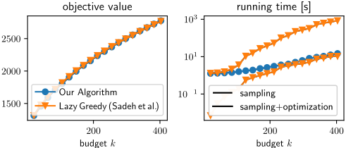
(weights sum to > 1). We compare our Algorithm 5 with Sadeh et al. [2020] (Algorithm 4). Results are in Figure 1 for τ = 5; see the full version for τ ∈ {10, n}. These are the largest networks in the literature for such models.
Discussion: Our Alg. 5 suffers only a small decrease in objective value while taking substantially fewer samples and running faster. For large budgets, our algorithm uses 10x fewer samples and is 200x faster.
4.2 Influence maximization on observed cascades
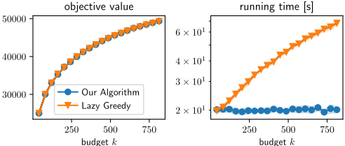
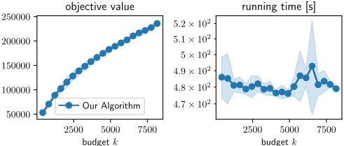
We obtain a single graph Gi = (V, Ei) by including (u, v) ∈ Ei with probability 1 deg(u) for each directed edge (u, v) ∈ E. We sample ℓ = 100 such graphs independently to form the observed cascades instance. Table 1 shows the total number of edges mtot. We use Algorithm 9 and estimate influence via Algorithm 7 for unrestricted (τ = n) and Algorithm 8 for restricted influence (τ < n). We compare with the greedy algorithm with lazy evaluations, the state of the art with theoretical guarantees; all other such algorithms are for stochastic models [Tang et al., 2015; Guo et al., 2022]. Figures 2 and 3 show results for the Twitter and Pokec networks and we provide further results in the full version. Lazy greedy does not scale to Pokec and Google-Plus instances, so we exclude it.
Discussion: Our algorithm vastly outperforms lazy greedy in running time while achieving nearly the same objective value, and easily scales to networks like Pokec with 100M edges, requiring only a few minutes even for large budgets. Additional experimental results, including further datasets, parameter settings, and diffusion step values, are provided in the full version.
5 Conclusion
We extend the low-adaptivity greedy framework of Chen et al. [2021b] to work with stochastic estimates of marginal gains, which is non-trivial since individual samples lack submodularity. We develop new estimation techniques: medianof-means with known variance bounds, an adaptive empirical variance estimator that avoids pessimistic worst-case bounds, and sketch-based estimators for observed cascades. For IC models, we prove a concentration bound replacing n with τ in sample complexity. These yield improved complexity, faster running time, and scalability, including the first nearly-linear algorithm for observed cascades with provable guarantees. Experiments confirm substantial speedups while maintaining near-optimal solution quality.
Acknowledgements
- FS was supported in part by NSF CAREER grant CCF1750333. TH was supported in part by an Alfred P. Sloan Research Fellowship. AE was supported in part by NSF CAREER grant CCF-1750333 and an Alfred P. Sloan Research Fellowship. HN was supported in part by NSF grant CCF2311649. We thank Ta Duy Nguyen for helpful discussions in the preliminary stages of this work.
@inproceedings{ijcai2026p40,
  title     = {Efficient Algorithms for Influence Maximization in General Models and Observed Cascades},
  author    = {Spaeh, Fabian and Haris, Themistoklis and Ene, Alina and Nguyen, Huy L.},
  booktitle = {Proceedings of the Thirty-Fifth International Joint Conference on
               Artificial Intelligence, {IJCAI-26}},
  publisher = {International Joint Conferences on Artificial Intelligence Organization},
  editor    = {Diego Calvanese},
  pages     = {348--356},
  year      = {2026},
  month     = {8},
  note      = {Main Track},
  doi       = {10.24963/ijcai.2026/40},
  url       = {https://doi.org/10.24963/ijcai.2026/40},
}
TY - CPAPER TI - Efficient Algorithms for Influence Maximization in General Models and Observed Cascades AU - Spaeh, Fabian AU - Haris, Themistoklis AU - Ene, Alina AU - Nguyen, Huy L. T2 - Proceedings of the Thirty-Fifth International Joint Conference on Artificial Intelligence, IJCAI-26 PB - International Joint Conferences on Artificial Intelligence Organization PY - 2026 SP - 348 EP - 356 DO - 10.24963/ijcai.2026/40 UR - https://doi.org/10.24963/ijcai.2026/40 ER -Copied
Machine-readable versions of this paper, for tools and AI agents:





