
H²SCAN: Adaptive Time Series Representation Learning via Heterogeneous Hypergraph Structure-aware Contrasts
Proceedings of the Thirty-Fifth International Joint Conference on Artificial Intelligence. Main Track. Pages 2465-2473.
https://doi.org/10.24963/ijcai.2026/274
Keywords
- Data Mining: Mining spatial and/or temporal data
- Knowledge Representation and Reasoning: Qualitative, geometric, spatial, and temporal reasoning
- Data Mining: Parallel, distributed and cloud-based high performance mining
- Machine Learning: Self-supervised Learning
- Data Mining: Mining heterogenous data
Abstract
Learning universal representations for time series is fundamental for diverse downstream tasks. However, current approaches largely rely on handcrafted data augmentations, which may distort intrinsic temporal dynamics and structural regularities. In addition, most static representation learning frameworks struggle to cope with the non-stationary nature of real-world time series. To address these issues, we propose Heterogeneous Hypergraph Structure-aware Contrastive Adaptive Network (H²SCAN), a novel augmentation-free framework that derives contrastive supervision directly from graph topology. Specifically, H²SCAN constructs a heterogeneous hypergraph with three node types to capture multi-scale temporal characteristics. Building upon this representation, a meta-adaptation network is introduced to dynamically reweight heterogeneous hyperedges, enabling the model to adapt to distribution shifts in real-time. Finally, a structure-aware contrastive learning objective is employed to align latent representation similarity with the intrinsic hypergraph topology. Experiments on multiple benchmarks and cloud Kafka cluster datasets demonstrate that H²SCAN outperforms existing methods by modeling high-order multi-domain dependencies and preserving the semantic integrity of time series data.
- [Andrzejak et al., 2001] Ralph G Andrzejak, Klaus Lehn- ertz, Florian Mormann, Christoph Rieke, Peter David, and Christian E Elger. Indications of nonlinear deterministic and finite-dimensional structures in time series of brain electrical activity: Dependence on recording region and brain state. PRE, 64(6):061907, 2001.
- [Anguita et al., 2013] Davide Anguita, Alessandro Ghio, Luca Oneto, Xavier Parra, Jorge Luis Reyes-Ortiz, et al. A public domain dataset for human activity recognition using smartphones. In Esann, volume 3, pages 3-4, 2013.
- [Cai et al., 2025] Ruichu Cai, Zhifan Jiang, Kaitao Zheng, Zijian Li, Weilin Chen, Xuexin Chen, Yifan Shen, Guangyi Chen, Zhifeng Hao, and Kun Zhang. Learning disentangled representation for multi-modal time-series sensing signals. In WWW, pages 3247-3266, 2025.
- [Chang et al., 2024] Ching Chang, Chiao-Tung Chan, Wei- Yao Wang, Wen-Chih Peng, and Tien-Fu Chen. Time- drl: Disentangled representation learning for multivariate time-series. In ICDE, pages 625-638, 2024.
- [Chen et al., 2020] Ting Chen, Simon Kornblith, Moham- mad Norouzi, and Geoffrey Hinton. A simple framework for contrastive learning of visual representations. In ICML, pages 1597-1607, 2020.
- [Cheng et al., 2025] Rui Cheng, Xiangfei Jia, Qing Li, Rong Xing, Jiwen Huang, Yu Zheng, and Zhilong Xie. Fat: Frequency-aware pretraining for enhanced time-series rep- resentation learning. In SIGKDD, pages 310-321, 2025.
- [Dau et al., 2019] Hoang Anh Dau, Anthony Bagnall, Kaveh Kamgar, Chin-Chia Michael Yeh, Yan Zhu, Shaghayegh Gharghabi, Chotirat Ann Ratanamahatana, and Eamonn Keogh. The ucr time series archive. JAS, 6(6):1293-1305, 2019.
- [Demirel and Holz, 2025] Berken Utku Demirel and Chris- tian Holz. Learning without augmenting: Unsupervised time series representation learning via frame projections. NeurIPS, 2025.
- [Dong et al., 2023] Jiaxiang Dong, Haixu Wu, Haoran Zhang, Li Zhang, Jianmin Wang, and Mingsheng Long. Simmtm: A simple pre-training framework for masked time-series modeling. NeurIPS, 36:29996-30025, 2023.
- [Eldele et al., 2021] Emadeldeen Eldele, Mohamed Ragab, Zhenghua Chen, Min Wu, Chee Keong Kwoh, Xiaoli Li, and Cuntai Guan. Time-series representation learning via temporal and contextual contrasting. IJCAI, 2021. IJCAI
- [Eldele et al., 2023] Emadeldeen Eldele, Mohamed Ragab, Zhenghua Chen, Min Wu, Chee-Keong Kwoh, Xiaoli Li, and Cuntai Guan. Self-supervised contrastive represen- tation learning for semi-supervised time-series classifica- tion. TPAMI, 45(12):15604-15618, 2023.
- [Fu and Hu, 2025] En Fu and Yanyan Hu. Frequency- masked embedding inference: A non-contrastive approach for time series representation learning. In AAAI, vol- ume 39, pages 16639-16647, 2025.
- [Germain et al., 2025] Thibaut Germain, Chrysoula Kosma, and Laurent Oudre. Time series representations with hard- coded invariances. In ICML, 2025.
- [Goldberger et al., 2000] Ary L Goldberger, Luis AN Ama- ral, Leon Glass, Jeffrey M Hausdorff, Plamen Ch Ivanov, Roger G Mark, Joseph E Mietus, George B Moody, Chung-Kang Peng, and H Eugene Stanley. Physiobank, physiotoolkit, and physionet: components of a new re- search resource for complex physiologic signals. circu- lation, 101(23):e215-e220, 2000.
- [Han et al., 2021] Peng Han, Jin Wang, Di Yao, Shuo Shang, and Xiangliang Zhang. A graph-based approach for tra- jectory similarity computation in spatial networks. In SIGKDD, pages 556-564, 2021.
- [He et al., 2022] Kaiming He, Xinlei Chen, Saining Xie, Yanghao Li, Piotr Dollár, and Ross Girshick. Masked au- toencoders are scalable vision learners. In CVPR, pages 16000-16009, 2022.
- [Kara et al., 2025] Denizhan Kara, Tomoyoshi Kimura, Jinyang Li, Bowen He, Yizhuo Chen, Yigong Hu, Hongjue Zhao, Shengzhong Liu, and Tarek F Abdelzaher. Adats: Learning adaptive time series representations via dynamic soft contrasts. In NeurIPS, 2025.
- [Lessmeier et al., 2016] Christian Lessmeier, James Kuria Kimotho, Detmar Zimmer, and Walter Sextro. Condition monitoring of bearing damage in electromechanical drive systems by using motor current signals of electric motors: A benchmark data set for data-driven classification. In PHME, volume 3, 2016.
- [Li et al., 2017] Yaguang Li, Rose Yu, Cyrus Shahabi, and Yan Liu. Diffusion convolutional recurrent neural net- work: Data-driven traffic forecasting. ICLR, 2017.
- [Li et al., 2023] Zhe Li, Zhongwen Rao, Lujia Pan, Pengyun Wang, and Zenglin Xu. Ti-mae: Self-supervised masked time series autoencoders. arXiv preprint arXiv:2301.08871, 2023.
- [Li et al., 2025] Boyuan Li, Yicheng Luo, Zhen Liu, Junhao Zheng, Jianming Lv, and Qianli Ma. Hyperimts: Hyper- graph neural network for irregular multivariate time series forecasting. ICML, 2025.
- [Liang et al., 2024] Yuxuan Liang, Haomin Wen, Yuqi Nie, Yushan Jiang, Ming Jin, Dongjin Song, Shirui Pan, and Qingsong Wen. Foundation models for time series analy- sis: A tutorial and survey. In SIGKDD, pages 6555-6565, 2024.
- [Liu and Chen, 2024] Jiexi Liu and Songcan Chen. Timesurl: Self-supervised contrastive learning for universal time series representation learning. In AAAI, volume 38, pages 13918-13926, 2024.
- [Liu et al., 2009] Jiayang Liu, Lin Zhong, Jehan Wickrama- suriya, and Venu Vasudevan. uwave: Accelerometer- based personalized gesture recognition and its applica- tions. PMC, 5(6):657-675, 2009.
- [Luo et al., 2023] Dongsheng Luo, Wei Cheng, Yingheng Wang, Dongkuan Xu, Jingchao Ni, Wenchao Yu, Xuchao Zhang, Yanchi Liu, Yuncong Chen, Haifeng Chen, et al. Time series contrastive learning with information-aware augmentations. In AAAI, volume 37, pages 4534-4542, 2023.
- [Nie, 2022] Y Nie. A time series is worth 64words: Long- term forecasting with transformers. ICLR, 2022.
- [Saxena et al., 2008] Abhinav Saxena, Kai Goebel, Don Si- mon, and Neil Eklund. Damage propagation modeling for aircraft engine run-to-failure simulation. In PHM, pages 1-9, 2008.
- [Wang et al., 2018] Biao Wang, Yaguo Lei, Naipeng Li, and Ningbo Li. A hybrid prognostics approach for estimating remaining useful life of rolling element bearings. IEEE Transactions on Reliability, 69(1):401-412, 2018.
- [Wang et al., 2024] Daoyu Wang, Mingyue Cheng, Zhiding Liu, and Qi Liu. Timedart: A diffusion autoregressive transformer for self-supervised time series representation. ICML, 2024.
- [Wiliński et al., 2024] Michał Wiliński, Mononito Goswami, Willa Potosnak, Nina Żukowska, and Artur Dubrawski. Exploring representations and interventions in time series foundation models. ICML, 2024.
- [Woo et al., 2022] Gerald Woo, Chenghao Liu, Doyen Sa- hoo, Akshat Kumar, and Steven Hoi. Cost: Contrastive learning of disentangled seasonal-trend representations for time series forecasting. ICLR, 2022.
- [Wu et al., 2022] Haixu Wu, Tengge Hu, Yong Liu, Hang Zhou, Jianmin Wang, and Mingsheng Long. Timesnet: Temporal 2d-variation modeling for general time series analysis. ICLR, 2022.
- [Yang et al., 2023] Yiyuan Yang, Chaoli Zhang, Tian Zhou, Qingsong Wen, and Liang Sun. Dcdetector: Dual attention contrastive representation learning for time series anomaly detection. In SIGKDD, pages 3033-3045, 2023.
- [Yu et al., 2017] Bing Yu, Haoteng Yin, and Zhanxing Zhu. Spatio-temporal graph convolutional networks: A deep learning framework for traffic forecasting. IJCAI, 2017. IJCAI
- [Yue et al., 2022] Zhihan Yue, Yujing Wang, Juanyong Duan, Tianmeng Yang, Congrui Huang, Yunhai Tong, and Bixiong Xu. Ts2vec: Towards universal representation of time series. In AAAI, volume 36, pages 8980-8987, 2022.
- [Zerveas et al., 2021] George Zerveas, Srideepika Jayara- man, Dhaval Patel, Anuradha Bhamidipaty, and Carsten Eickhoff. A transformer-based framework for multivari- ate time series representation learning. In SIGKDD, pages 2114-2124, 2021.
- [Zhang et al., 2022] Xiang Zhang, Ziyuan Zhao, Theodoros Tsiligkaridis, and Marinka Zitnik. Self-supervised con- trastive pre-training for time series via time-frequency consistency. NeurIPS, 35:3988-4003, 2022.
- [Zhang et al., 2024] Kexin Zhang, Qingsong Wen, Chaoli Zhang, Rongyao Cai, Ming Jin, Yong Liu, James Y Zhang, Yuxuan Liang, Guansong Pang, Dongjin Song, et al. Self- supervised learning for time series analysis: Taxonomy, progress, and prospects. TPAMI, 46(10):6775-6794, 2024.
References were extracted automatically from the PDF and may contain errors.
Full text extracted automatically from the PDF; figures, tables and equations may differ. The PDF is the version of record.
1 Introduction
Time series (TS) data pervades diverse domains, including industrial systems, healthcare monitoring, financial markets, and climate science [Yang et al., 2023; Liang et al., 2024]. Learning effective representations from TS is fundamental to enabling downstream tasks such as classification, forecasting, and anomaly detection [Wili´nski et al., 2024; Germain et al., 2025]. Nevertheless, labeled TS data remain inherently limited: annotation is often costly, time-consuming, and dependent on specialized domain expertise. This has spurred interest in self-supervised learning (SSL) for learning representations from unlabeled data [Eldele et al., 2023; Zhang et al., 2024; Wang et al., 2024; Cai et al., 2025].
Recent advances in SSL have been dominated by two paradigms: contrastive learning [Chen et al., 2020] and generative modeling [Zerveas et al., 2021; He et al., 2022]. Contrastive methods learn representations by maximizing agreement between differently augmented views of the same sample while distinguishing them from other samples. Generative methods, such as masked reconstruction, learn to predict missing or corrupted portions of the input [Nie, 2022]. While both approaches have shown promise, they face multiple limitations when applied to TS data [Wu et al., 2022].
L1: Non-Stationary Dynamics. TS data often exhibit pronounced non-stationarity with their distinctive multi-scale temporal dynamics and frequency-domain periodicity. As a typical TS example, the electrocardiogram (ECG) signal shown in Figure 1 (a) contains three distinct segments with dramatically different characteristics: Segment A exhibits high-frequency oscillations with low variance, Segment B displays low-frequency patterns with high amplitude, and Segment C shows mixed dynamics with trend shifts. However, existing approaches rely on monolithic or fixed architectures, limiting their adaptability to diverse temporal patterns and dynamic variations in the data.
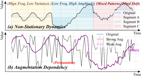
L2: Augmentation Dependency. Current contrastive methods rely heavily on data augmentation to construct positive/negative pairs. As illustrated in Figure 1 (b), strong augmentations (red line), such as temporal permutation, destroy the sequential order and temporal dependencies that define meaningful patterns. In our ECG example, permuting time steps scrambles the cardiac cycle structure, producing semantically invalid signals; Weak augmentations (purple line), such as additive noise, generate views too similar to the original, providing minimal contrastive signal for learning discriminative representations. These imposed artificial representational invariances may not align with the true invariances in the data, limiting generalization [Demirel and Holz, 2025].
Although existing methods have made notable progress in addressing L1 or L2 under specific scenarios, their reliance on fixed modeling paradigms leads to a limited domain perspective [Kara et al., 2025; Cheng et al., 2025]. As a result, global periodic structures in the frequency domain and distributional shifts in the statistical domain are often overlooked. For instance, in cloud Kafka clusters, monitoring models can neither distinguish transient spikes from systemic failures, thus falling into "alert fatigue", nor detect routine periodic features visible only in the frequency domain, such as scheduled batch jobs or log rotations. Moreover, critical distributional shifts, including data skew or hot partitions, often remain undetected due to limited statistical awareness.
To overcome these intertwined challenges, we propose H 2 SCAN, a unified framework that naturally captures the multi-faceted nature of TS while providing structural similarity for contrastive learning. Specifically, H 2 SCAN begins by constructing a heterogeneous hypergraph that integrates time, frequency, and statistics-aware nodes to capture multi-domain characteristics, with hyperedges modeling higher-order interactions beyond standard pairwise relationships. For L1, we introduce a meta-learning network that leverages segment-level statistics to adaptively reweight heterogeneous hyperedges, allowing the model to emphasize relevant cross-domain information under non-stationary dynamics without manual intervention. Moreover, these components are unified through a message passing mechanism that facilitates effective information propagation across the hypergraph, enabling rich multi-scale representation. For L2, we eliminate augmentation dependency by deriving soft similarity targets directly from hypergraph topology, where samples with similar structural patterns are naturally aligned, enabling the encoder to be trained with continuous similarity scores instead of hard positive/negative pairs.
Our main contributions are summarized as follows:
- We introduce a hypergraph architecture that simultaneously models temporal, frequency, and statistical characteristics of time series.
- We propose a meta-adaptation mechanism that generates instance-specific weights for hypergraph message passing, enabling real-time adaptation to distribution shifts.
- We design a soft contrastive objective that uses hypergraph topological similarity as a natural supervision signal, bypassing the pitfalls of manual data augmentation.
- Extensive experiments on various datasets demonstrate H 2 SCAN outperforms state-of-the-art methods, showcasing the benefits of multi-domain structural modeling. Additionally, we construct four cloud cluster datasets to explore TSRL in elastic message-queue scaling.
2 RelatedWork
Time Series Representation Learning. Traditional methods focused on learning instance-level representations using recurrent architectures, but recent advances have shifted toward self-supervised contrastive learning paradigms. TS-TCC [Eldele et al., 2021] proposes a temporal and contextual contrasting framework that learns robust representations by utilizing strong and weak augmentations. To capture multiscale features, TS2Vec [Yue et al., 2022] introduces a hierarchical contrastive framework capable of learning improved representations across various semantic levels. Addressing the frequency domain, CoST [Woo et al., 2022] and TF-C [Zhang et al., 2022] leverage spectral information to disentangle seasonal and trend components, thereby preserving complex temporal dynamics. Beyond contrastive methods, generative approaches inspired by masked image modeling have gained traction. Ti-MAE [Li et al., 2023] applies a masked autoencoder architecture to TS, demonstrating strong generalization capabilities. To mitigate the difficulty of reconstruction in high-noise environments, SimMTM [Dong et al., 2023] proposes a manifold-aware masked modeling strategy that reconstructs the original series by aggregating information from multiple neighbors, effectively guiding the learning process in a low-dimensional manifold.
Using Graphs for Time Series. Modeling TS as graphs captures complex inter-dependencies between variables. Early works like DCRNN [Li et al., 2017] and STGCN [Yu et al., 2017] integrate Graph Neural Networks (GNNs) with recurrent or convolutional layers to model spatial and temporal dependencies simultaneously, primarily relying on pre-defined graph structures. Recent research focuses on capturing dynamic correlations. GTS [Han et al., 2021] utilizes a discrete graph structure learning mechanism to infer probabilistic dependencies between TS online.
3 ProblemDefinition
Consider a TS dataset D = {Ti}Ni=1 , where each sample Ti ∈ RT×C consists of C variables recorded over T timestamps. To capture the complex interactions across different domains, H 2 SCAN formally map each sample Ti to a heterogeneous hypergraph Gi = (Vi, Ei,Wi), where Vi denotes the set of multi-domain nodes, Ei represents the set of multi-type hyperedges, and Wi contains the adaptive hyperedge weights predicted by a meta-learner.
Our goal is to learn a universal encoder fθ : RT×C → Rd that maps an input series Ti to a d-dimensional latent representation Zi. This encoder is optimized via a two-stage paradigm: ❶ In the pre-training phase, we aim to optimize fθ by minimizing a joint loss L = Lcl + λLrec. Here, Lrec is a reconstruction loss, Lcl is a structural contrastive loss that aligns the representation similarity Srepr(Zi,Zj) with the hypergraph structural similarity Sstruct(Gi, Gj):
where Pstruct/repr(j|i) is the normalized similarity distribution. ❷ In the fine-tuning phase, the pre-trained encoder fθ is adapted to specific tasks using a task-specific head gϕ.
4 Methodology
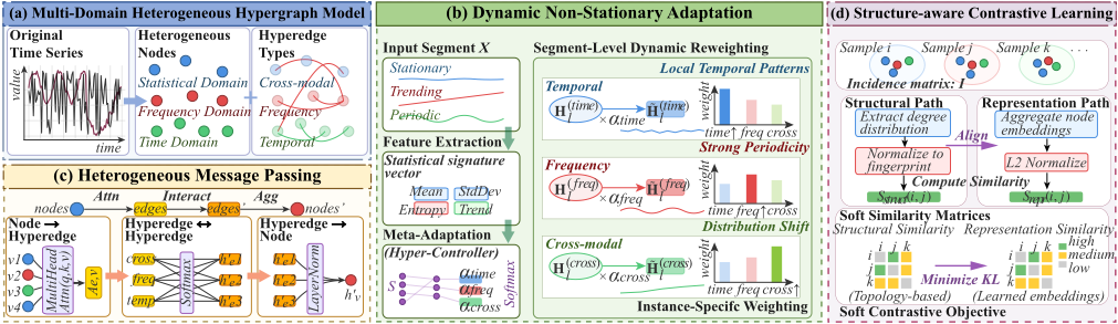
Figure 2 shows the framework of H 2 SCAN, which consists of the following four major modules:
- Multi-domain Heterogeneous Hypergraph Modeling, which represents TS across complementary information spaces by explicitly encoding time, frequency, and statistical domains as heterogeneous nodes connected via multi-type hyperedges (Section 4.1).
- Dynamic Non-stationary Adaptation, which learns data-driven hyperedge weighting functions to model diverse temporal dynamics beyond fixed architectures, enabling the hypergraph structure to adjust to evolving TS characteristics (Section 4.2).
- Heterogeneous Message Passing, which propagates information across multi-domain hypergraph structures through structure-aware attention and cross-type interactions (Section 4.3).
- Structure-aware Contrastive Learning, which replaces augmentation-dependent similarity construction with topology-driven supervision by deriving soft similarity targets directly from the intrinsic multi-domain hypergraph structure (Section 4.4).
4.1 Multi-Domain Heterogeneous Hypergraph Construction
This work proposes a heterogeneous hypergraph architecture that explicitly models TS across multiple information domains, as shown in Figure 2 (a).
Heterogeneous Node Types. Instead of embedding TS into a single latent space, we project each sample T into three distinct feature spaces. i) Time-Domain Nodes. For the capture of local temporal patterns, we encode each observation using a convolutional encoder:
where ϕtime consists of 1D convolutions with batch normalization. This produces L time-domain nodes vtime t for t = 1, . . . ,L. ii) Frequency-Domain Nodes. In order to capture global periodic patterns, we extract frequency components via the FFT: F = FFT(T ). Complex coefficients are then decomposed into real and imaginary parts and encoded:
where Nf = L/2 + 1 represents the number of frequency modes, and ϕfreq : R2 →Rd is a linear projection.
iii) Statistical Nodes. Summary statistics are computed to capture distributional properties and high-level characteristics: S = [µ(T ), σ(T ),min(T ),max(T )], where µ and σ denote mean and standard deviation across the entire series. Statistical nodes are encoded as:
The complete heterogeneous node set is: V = V time ∪ V freq ∪ V stat with total N = L + Nf + 4 nodes.
Multi-Type Hyperedge Design. Hypergraphs model higherorder interactions where multiple hyperedges participate simultaneously. i) Temporal Hyperedges. To capture shortterm dependencies, temporal hyperedges E temp connect timedomain nodes within local temporal neighborhoods: etemp t = {vtime i : |i - t| ≤ w}, where w is the temporal window size. The hyperedge representation is then computed via attention-based aggregation: htemp t = ϕtemp (∑v∈etemp t αt,vv), where αt,v are learnable attention weights. ii) Frequency Hyperedges. Frequency hyperedges E freq connect frequencydomain nodes with coherent spectral characteristics: efreq k = {vfreq i : i ∈ Nk}, where Nk contains frequency indices with similar magnitudes or harmonically related frequencies. This hyperedge embedding is: hfreq βk,vv).
k = ϕfreq (∑v∈efreq k iii) Cross-Modal Hyperedges. Cross-modal hyperedges E cross bridge different node types to enable information flow across domains: ecross j = {vtime i , vfreq k , vstat m }. Each E cross connects nodes from all three domains, with representation: hcross j = ϕcross (⊕v∈ecross j γj,vv), where ⊕ denotes concatena-
tion, and γj,v are domain-specific attention weights.
The hypergraph structure is then formally captured by incidence matrices H(type) ∈ {0, 1}|E(type) |×N for each type of hyperedge:
The complete hypergraph is represented as G = (V, E temp ∪ E freq ∪ E cross , {H(type) }).
4.2 Dynamic Non-Stationary Adaptation
A dynamic adaptation mechanism that reconfigures the hypergraph's focus based on the real-time characteristics of the input data is introduced as shown in Figure 2 (b).
Meta-Adaptation Network. A meta-adaptation network Mθ acts as a hyper-controller for the model, predicting instance-specific weights for each hyperedge type conditioned on the input's statistical signature.
For an input segment T ∈ RT×C , we first extract a statistical feature vector s ∈ R4 that encapsulates the segment's distributional and spectral properties:
where µ(T ) and σ(T ) are the mean and standard deviation, capturing basic distribution properties. Hspec(T ) is the spectral entropy, computed from the normalized power spectrum of the FFT, quantifying the signal's complexity and periodicity. βtrend(T ) is the linear trend coefficient, capturing the directional evolution of the series.
The meta-network processes s through a multi-layer perceptron to generate the adaptive weight vector α:
which determines the relative importance of temporal, frequency, and cross-modal information.
Segment-Level Dynamically Reweighting. The learned adaptive weights α are applied directly during the message passing phase (detailed in Section 4.3) to modulate information flow. This allows the model to dynamically shift its inductive bias: effectively paying attention to frequency coherence when periodicities are strong (high αfreq), or focusing on statistical stability during distribution shifts (high αcross).
Formally, let H(type) l denote the aggregated hyperedge representations for a specific type at layer l. The dynamic reweighting is applied prior to node updates as:
where type is constrained to the set {time, freq, cross}.
4.3 Heterogeneous Message Passing
For the propagation of information from the crosshypergraph, a multi-stage message transmission mechanism is designed as shown in Figure 2 (c).
Node-to-Hyperedge Attention. First, we aggregate information from nodes to their connected hyperedges. A multihead attention mechanism that dynamically weighs the contribution of each node based on its semantic relevance is employed. For a hyperedge e ∈ E and its connected nodes N(e), the hyperedge representation he ∈ Rd is updated as:
where h(0) e is the initial hyperedge embedding serving as the query, and HV represents the matrix of node features serving as keys and values.
To ensure that only structurally connected nodes contribute to the hyperedge representation, the attention mechanism then utilizes the incidence matrix I to mask irrelevant nodes:
Hyperedge-to-Hyperedge Interaction. To capture higherorder dependencies beyond direct node connections, we introduce an interaction layer among hyperedges.
Representations from all hyperedge types are concatenated into a unified set HE = [Htime;Hfreq;Hcross]. We then apply an irregularity-aware attention mechanism to model the dependencies between these hyperedges:
where QE , KE , VE are linear projections of HE .
Hyperedge-to-Node Aggregation. Finally, we propagate the refined hyperedge information back to the nodes to update their representations. For a node v, its updated representation h′v is computed by aggregating information from all hyperedges e connected to it, weighted by the incidence matrix I:
The node update incorporates a residual connection and layer normalization for training stability:
This completes one layer of heterogeneous message passing [Li et al., 2025], fusing multi-domain information into a unified representation for downstream tasks.
4.4 Structure-aware Contrastive Learning
As shown in Figure 2 (d), a structure-aware contrastive learning framework leverages the intrinsic connectivity of the heterogeneous hypergraph to define pairwise similarities.
Hypergraph Structural Similarity. The structural equivalence between samples is quantified based on their connectivity patterns within the hypergraph topology. Two TS samples are similar if they exhibit similar connectivity patterns.
A structural fingerprint fi ∈ R|V| for the i-th sample is defined based on its node degree distribution across all hyperedge types. Let I ∈ R|E|×|V| be the aggregated incidence matrix. The degree vector di for sample i is computed by summing connections across all hyperedges:
The structural fingerprint is obtained by normalizing the degree vector to form a probability distribution:
The structural similarity Sstruct(i, j) between sample i and sample j is then computed as the cosine similarity between their fingerprints:
Representation Similarity. Similarity in the learned latent space is computed concurrently. Let zi ∈ Rd be the global representation of sample i, obtained by aggregating its constituent node embeddings:
The representation similarity Srepr(i, j) is defined as the cosine similarity between the normalized embedding vectors:
Soft Contrastive Objective. To align the learned representation space with the structural topology, we employ a soft contrastive objective. The structural similarity distribution serves as a soft target rather than binary labels.
Both similarity matrices are converted into probability distributions using a temperature parameter τ :
The objective is to minimize the Kullback-Leibler divergence between the predicted representation distribution and the target structural distribution:
where Pstruct(·|i) and Prepr(·|i) represent the structural and the latent representation similarity distribution, respectively.
5 Experiments
In this section, we conduct comprehensive experiments to evaluate the effectiveness of H 2 SCAN:
- RQ1: How does H 2 SCAN perform compared with existing TSRL methods?
- RQ2: How does every component that we design contribute to the overall performance?
- RQ3: How sensitive is H 2 SCAN to variations in key parameter settings?
- RQ4: How does the computational efficiency of H 2 SCAN compare to the baselines?
5.1 Experimental Setup
Datasets. The experiments are conducted on 12 realworld datasets, four self-built cloud Kafka cluster datasets constructed for both classification and regression tasks across broker-level and topic-level components, with detailed statistics reported in Table 1. The cloud Kafka cluster datasets are collected from a 5-broker cloud cluster (September-December 2025), comprising KCluster-broker with seven broker-level metrics and KCluster-topic with topic-level traffic, storage, and request-handling metrics. In addition, eight well-established public datasets are used, including Gesture [Liu et al., 2009], FD-B [Lessmeier et al., 2016], EMG [Goldberger et al., 2000], EPI [Andrzejak et al., 2001], HAR [Anguita et al., 2013], and UCR [Dau et al.,
| Tasks | Datasets | Samples | Length | Freq. | Classes |
|---|---|---|---|---|---|
| Clas. | KCluster-bc | 2,163 | 178 | 2 Hours | 5 |
| KCluster-tc | 2,163 | 178 | 2 Hours | 7 | |
| Reg. | KCluster-br | 1,384/346/433 | 35 | 2 Hours | - |
| KCluster-tr | 1,384/346/433 | 35 | 2 Hours | - |
2019] for classification, and C-MAPSS [Saxena et al., 2008] and Bearing [Wang et al., 2018] for regression.
Baselines. To evaluate the effectiveness of the proposed H 2 SCAN, we implement in total seven baselines: i) FEI [Fu and Hu, 2025] leverages frequency-masked prompts to model continuous semantics without explicit positive/negative pairs. ii) TimeDRL [Chang et al., 2024] learns dual-level disentangled embeddings for multivariate TS via a token-based strategy. iii) TimesURL [Liu and Chen, 2024] captures segmentand instance-level information by injecting double Universums as hard negatives. iv) SimMTM [Dong et al., 2023] connects masked modeling with manifold learning by reconstructing series from aggregated masked variants. v) InfoTS [Luo et al., 2023] adaptively selects data augmentations using information-theoretic criteria. vi) TF-C [Zhang et al., 2022] enforces time-frequency consistency through crossspace projectors and a joint loss. vii) TS2Vec [Yue et al., 2022] performs hierarchical contrastive learning over augmented views to learn robust timestamp representations.
Implementation Details. All experiments were conducted using PyTorch 2.6.0 on a server with two Tesla V100 GPUs, 128GB RAM, and a 12-core CPU. We optimized the models using the Adam optimizer with a learning rate of 5e-4 and a batch size of 512, training for 150 epochs per data batch. For the specific modules within H 2 SCAN, the structural similarity threshold in Equation (16) is set to 0.5, and the adaptation function initial weight is set to 0.3.
5.2 Main Results (RQ1)
We compare H 2 SCAN with all seven baselines across multiple classification and regression benchmarks. Tables 2 and 3 list the results for two tasks.
Classification. The first observation is that H 2 SCAN achieves the best performance in terms of accuracy across all eight datasets. This confirms the superior capability of our framework in learning discriminative representations by integrating multi-domain nodes during the pre-training phase. Specifically, H 2 SCAN achieves an average improvement of 2.89% over the strongest baseline FEI. Moreover, we observe that augmentation-based methods like TS2Vec, TimeDRL, and TimesURL perform relatively poorly on datasets with sensitive periodic signatures, such as EMG and KClustertc. This is likely because their manual perturbations distort the underlying frequency components and physical laws of the TS. The third observation is that while frequencyaware methods like TF-C and FEI capture periodic patterns, H 2 SCAN offers a key advantage by using cross-modal hyperedges to fuse these patterns with global statistical context, leading to more robust classifications in complex cloud scenarios where data noise is prevalent.
| Datasets | Rand. Init. | TS2Vec | TimeDRL | TF-C | TimesURL | SimMTM | InfoTS | FEI | H 2 SCAN |
|---|---|---|---|---|---|---|---|---|---|
| Gesture | 68.33 | 72.50 | 73.33 | 70.00 | 73.33 | 76.67 | 71.67 | 77.50 | 78.33 |
| FD-B | 69.61 | 48.31 | 47.97 | 65.48 | 54.41 | 63.49 | 62.99 | 70.99 | 71.38 |
| EMG | 95.12 | 78.05 | 78.05 | 92.68 | 73.17 | 87.80 | 97.56 | 97.56 | 97.56 |
| EPI | 80.21 | 95.60 | 94.05 | 95.28 | 96.67 | 96.22 | 97.07 | 97.24 | 97.30 |
| HAR | 82.66 | 64.74 | 79.88 | 77.27 | 77.57 | 83.61 | 82.49 | 84.15 | 84.97 |
| UCR | 72.44 | 67.44 | 63.36 | 78.50 | 79.40 | 80.42 | 81.77 | 82.65 | 82.71 |
| KCluster-bc | 72.02 | 72.02 | 77.52 | 66.51 | 71.04 | 74.77 | 72.02 | 69.27 | 83.95 |
| KCluster-tc | 64.68 | 65.60 | 65.60 | 61.93 | 66.51 | 61.93 | 61.01 | 65.59 | 67.43 |
| Avg. | 75.63 | 70.53 | 72.47 | 75.96 | 74.01 | 78.11 | 78.32 | 80.62 | 82.95 |
| Datasets | Rand. Init. | TS2Vec | TimeDRL | TF-C | TimesURL | SimMTM | InfoTS | FEI | H 2 SCAN |
|---|---|---|---|---|---|---|---|---|---|
| C-MAPSS | 0.067 / 0.206 | 0.061 / 0.207 | 0.083 / 0.245 | 0.063 / 0.215 | 0.060 / 0.205 | 0.086 / 0.221 | 0.072 / 0.213 | 0.079 / 0.214 | 0.060 / 0.199 |
| Bearing | 0.073 / 0.184 | 0.184 / 0.265 | 0.147 / 0.289 | 0.604 / 0.645 | 0.164 / 0.256 | 0.054 / 0.140 | 0.073 / 0.178 | 0.033 / 0.115 | 0.030 / 0.109 |
| KCluster-br | 0.063 / 0.177 | 0.269 / 0.481 | 0.029 / 0.065 | 0.529 / 0.700 | 0.440 / 0.646 | 0.032 / 0.093 | 0.030 / 0.078 | 0.024 / 0.077 | 0.028 / 0.055 |
| KCluster-tr | 0.005 / 0.057 | 0.317 / 0.439 | 0.004 / 0.054 | 0.458 / 0.501 | 0.672 / 0.712 | 0.014 / 0.109 | 0.001 / 0.028 | 0.002 / 0.032 | 0.001 / 0.024 |
| Avg. | 0.052 / 0.156 | 0.208 / 0.348 | 0.066 / 0.163 | 0.414 / 0.515 | 0.334 / 0.455 | 0.047 / 0.141 | 0.044 / 0.124 | 0.035 / 0.110 | 0.030 / 0.097 |
| Metrics | MSE | MAE |
|---|---|---|
| H 2 SCAN w/o frequency w/o statistical w/o freq.+stat. | 0.0604 | 0.1987 |
| 0.0618 | 0.2078 | |
| 0.0612 | 0.2100 | |
| 0.0754 | 0.2140 | |
| w/o meta. | 0.0612 | 0.2093 |
Regression. H 2 SCAN also achieves the best regression performance across all datasets. A primary reason for this success is the introduction of the Meta-Adaptation Network, which allows H 2 SCAN to handle the non-stationary nature of industrial sensor data and cloud traffic. In remaining useful life prediction tasks, where statistical properties evolve as machinery degrades, H 2 SCAN dynamically reweights its hypergraph interactions to maintain predictive stability. Specifically, our model achieves an average error reduction of 16.89% compared to FEI and InfoTS. The performance advantage is particularly pronounced on the KCluster-tr dataset. This suggests that the high-order relationships captured by our hyperedge design are essential for modeling the intricate dependencies in distributed clusters.
5.3 Ablation Study (RQ2)
In the ablation study, we quantify the contribution of each H 2 SCAN component. The results on the C-MAPSS dataset for regression are shown in Table 4, confirming the necessity of each module in the framework.
Experimental results of the four variants illustrate that the most significant performance decline occurs when both the frequency and statistical domains (w/o freq.+stat.) are excluded. This drop is due to the model's inability to capture global periodicities and distributional properties, forcing it to rely solely on local temporal sequences. Similarly, the individual removal of the frequency domain (w/o freq.) or the statistical domain (w/o stat.) leads to a noticeable decrease in predictive accuracy, highlighting the importance of multidomain feature integration for robust representation learning. Furthermore, excluding the meta-adaptation network (w/o meta.) results in performance degradation, as it disables the model's ability to dynamically reweight hyperedge interactions in response to the non-stationary nature of industrial sensor data.
5.4 Hyperparameter Sensitivity (RQ3)
Varying Hypergraph Layers. We investigate the impact of model depth by varying the number of hypergraph layers from 1 to 5. As shown in Figures 3 (a) and (b), it can be observed that the performance of H 2 SCAN remains relatively stable as the depth increases. Specifically, the best results are achieved with 4 layers for both datasets. H 2 SCAN captures high-order dependencies without requiring excessively deep architectures, demonstrating its robustness across varying model complexities.
Impact of Attention Heads. We analyze the influence of the number of attention heads used in the heterogeneous message passing module. Figures 3 (c) and (d) show results for heads in {2, 4, 6, 8, 10}. We observe that the choice of attention heads has a noticeable impact on the model's ability to capture multi-domain correlations. Specifically, the optimal performance is achieved when the number of heads is set to 8. This indicates that while multiple heads allow the model to attend to different semantic subspaces simultaneously, an excessive number of heads may introduce redundant information that slightly degrades the accuracy.
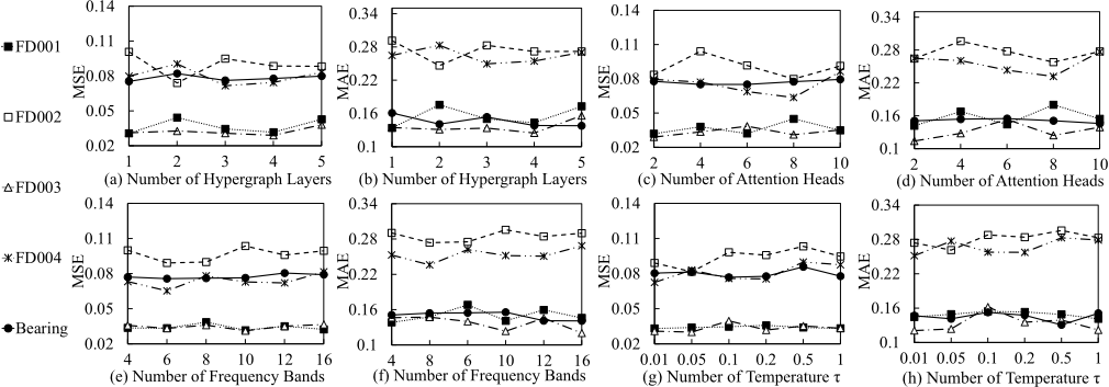
Selecting Frequency Bands b. We examine the parameter b, which determines the number of top frequency components selected for the frequency-domain nodes. Figures 3 (e) and (f) show the results for b values ranging from 4 to 16. We observe that b is a crucial factor in capturing the periodic signatures of industrial sensors. The C-MAPSS dataset, which contains complex turbofan engine data, benefits from a smaller b (set to 8), whereas the Bearing dataset, characterized by more distinct vibration frequencies, achieves peak performance with a larger b (set to 16). This suggests that H 2 SCAN can be tailored to the spectral complexity of the specific TS.
Effect of Temperature τ. H 2 SCAN utilizes a temperature parameter τ to control the sharpness of the soft contrastive distribution. We test various levels of τ, and the results are shown in Figures 3 (g) and (h). The model's performance is sensitive to the scale of similarity scores. A temperature of τ = 0.01 yields the best alignment between the representation space and the hypergraph topology. However, the impact of varying τ is relatively limited, with performance fluctuations controlled within 9.8%. This robustness is attributed to our structure-based contrastive objective, which provides a stable and natural supervision signal compared to traditional augmentation-based methods.
5.5 Efficiency Analysis (RQ4)
We evaluate the efficiency of each measure in both model pretraining time (per epoch) and end-to-end fine-tuning time. The experimental results are shown in Table 5. FEI distinguishes itself with the shortest pre-training time, attributed to its 1D ResNet-based encoder structure and the innovative frequency-masked embedding inference mechanism. In contrast, other models like TF-C and InfoTS consider additional complex contrastive pairs or frequency-time alignments that must be computed during pre-training, resulting in longer processing times. Our model, H 2 SCAN, although it includes complex components such as heterogeneous hypergraph modeling and a meta-adaptation network, still maintains high efficiency through optimized design. By utilizing sparse hypergraph message passing and efficient FFT-based frequency encoding, its pre-training time is only slightly longer than FEI and TS2Vec but achieves significantly higher accuracy in both classification and regression tasks. This indicates that H 2 SCAN successfully balances computational complexity and model effectiveness.
| Model | Pre-training time | Fine-tuning time |
|---|---|---|
| TS2Vec | 171.49 s | 4.78 s |
| TimeDRL | 426.95 s | 5.63 s |
| TF-C | 2120.15 s | 9.99 s |
| TimesURL | 650.71 s | 4.45 s |
| SimMTM | 517.57 s | 5.85 s |
| InfoTS | 1267.51 s | 19.16 s |
| FEI | 120.51 s | 7.61 s |
| H 2 SCAN | 212.09 s | 7.53 s |
6 Conclusion
In this paper, we propose H 2 SCAN, a structure-aware framework for time series representation learning. H 2 SCAN eliminates augmentation dependency by constructing multidomain heterogeneous hypergraphs, and leverages hypergraph topology as a natural source of similarity for contrastive learning. The meta-adaptation network enables dynamic adjustment to non-stationary patterns, while heterogeneous message passing captures higher-order multi-scale dependencies. Comprehensive empirical analyses validate that H 2 SCAN achieves state-of-the-art performance on twelve real-world datasets across diverse domains. The robustness and universality of H 2 SCAN make it a promising candidate for various practical applications.
Acknowledgments
This work was supported by the Natural Science Foundation of the National Natural Science Foundation of China under grant (No. 62572335), the National Key Research and Development Program of China (No.2023YFF0725002), Jiangsu Higher Education Institutions of China (No.23KJA520011), Enhancing Competitiveness through Data-Driven and Intelligent Process Optimization (No. SBC20071).
Contribution Statement
Biao Chen and Zijie Tang contributed equally. Junhua Fang is the corresponding author.
@inproceedings{ijcai2026p274,
  title     = {H²SCAN: Adaptive Time Series Representation Learning via Heterogeneous Hypergraph Structure-aware Contrasts},
  author    = {Chen, Biao and Tang, Zijie and Fang, Junhua and Lu, Feng and Zhang, Lang and Zhao, Pengpeng},
  booktitle = {Proceedings of the Thirty-Fifth International Joint Conference on
               Artificial Intelligence, {IJCAI-26}},
  publisher = {International Joint Conferences on Artificial Intelligence Organization},
  editor    = {Diego Calvanese},
  pages     = {2465--2473},
  year      = {2026},
  month     = {8},
  note      = {Main Track},
  doi       = {10.24963/ijcai.2026/274},
  url       = {https://doi.org/10.24963/ijcai.2026/274},
}
TY - CPAPER TI - H²SCAN: Adaptive Time Series Representation Learning via Heterogeneous Hypergraph Structure-aware Contrasts AU - Chen, Biao AU - Tang, Zijie AU - Fang, Junhua AU - Lu, Feng AU - Zhang, Lang AU - Zhao, Pengpeng T2 - Proceedings of the Thirty-Fifth International Joint Conference on Artificial Intelligence, IJCAI-26 PB - International Joint Conferences on Artificial Intelligence Organization PY - 2026 SP - 2465 EP - 2473 DO - 10.24963/ijcai.2026/274 UR - https://doi.org/10.24963/ijcai.2026/274 ER -Copied
Machine-readable versions of this paper, for tools and AI agents:





