
A Faster Deterministic Algorithm for Kidney Exchange via Representative Set
Proceedings of the Thirty-Fifth International Joint Conference on Artificial Intelligence. Main Track. Pages 2355-2363.
https://doi.org/10.24963/ijcai.2026/262
Keywords
- Game Theory and Economic Paradigms: Auctions and market-based systems
- Game Theory and Economic Paradigms: Computational social choice
- Constraint Satisfaction and Optimization: Constraint optimization problems
Abstract
The Kidney Exchange Problem is a prominent challenge in healthcare and economics, arising in the context of organ transplantation. It has been extensively studied in artificial intelligence and optimization. In a kidney exchange, a set of donor-recipient pairs and altruistic donors are considered, with the goal of identifying a sequence of exchanges—comprising cycles or chains starting from altruistic donors—such that each donor provides a kidney to the compatible recipient in the next donor-recipient pair. These exchanges create a network of transplants aimed at maximizing the total number, t, of successful transplants. Due to constraints in medical resources, limits are often imposed on the lengths of these cycles and chains. Recently, this problem was deterministically solved in O* (14.34ᵗ) time (IJCAI 2024). In this paper, we introduce the representative set technique for the Kidney Exchange Problem, showing that the problem can be deterministically solved in O* (6.855ᵗ) time.
- [Abraham et al., 2007] David J. Abraham, Avrim Blum, and Tuomas Sandholm. Clearing algorithms for barter ex- change markets: enabling nationwide kidney exchanges.
- In Jeffrey K. MacKie-Mason, David C. Parkes, and Paul Resnick, editors, Proceedings 8th ACM Conference on Electronic Commerce (EC-2007), San Diego, California, USA, June 11-15, 2007, pages 295-304. ACM, 2007.
- [Anderson et al., 2015] Ross Anderson, Itai Ashlagi, David Gamarnik, and Alvin E. Roth. Finding long chains in kid- ney exchange using the traveling salesman problem. Pro- ceedings of the National Academy of Sciences, 112:663 - 668, 2015.
- [Banik et al., 2025] Aritra Banik, Sujoy Bhore, Palash Dey, and Abhishek Sahu. Kidney exchange: Faster parameter- ized algorithms and tighter lower bounds, 2025.
- [Biró et al., 2009] Péter Biró, David F. Manlove, and Romeo Rizzi. Maximum weight cycle packing in directed graphs, with application to kidney exchange programs. Discret. Math. Algorithms Appl., 1(4):499-518, 2009.
- [Constantino et al., 2013] Miguel Constantino, Xenia Kli- mentova, Ana Viana, and Abdur Rais. New insights on integer-programming models for the kidney exchange problem. Eur. J. Oper. Res., 231(1):57-68, 2013.
- [Dickerson et al., 2016] John P. Dickerson, David F. Manlove, Benjamin Plaut, Tuomas Sandholm, and James Trimble. Position-indexed formulations for kidney ex- change. In Vincent Conitzer, Dirk Bergemann, and Yiling Chen, editors, Proceedings of the 2016 ACM Conference on Economics and Computation, EC '16, Maastricht, The Netherlands, July 24-28, 2016, pages 25-42. ACM, 2016.
- [Fomin et al., 2016] Fedor V. Fomin, Daniel Lokshtanov, Fa- had Panolan, and Saket Saurabh. Efficient computation of representative families with applications in parameterized and exact algorithms. J. ACM, 63(4):29:1-29:60, 2016.
- [Francis et al., 2024] Anna Francis, Meera N Harhay, Albert Ong, Sri Lekha Tummalapalli, Alberto Ortiz, Agnes B Fogo, Danilo Fliser, Prabir Roy-Chaudhury, Monica Fontana, Masaomi Nangaku, et al. Chronic kidney dis- ease and the global public health agenda: an international consensus. Nature Reviews Nephrology, pages 1-13, 2024.
- [Glorie et al., 2014] Kristiaan M. Glorie, Joris van de Klun- dert, and Albert P. M. Wagelmans. Kidney exchange with long chains: An efficient pricing algorithm for clear- ing barter exchanges with branch-and-price. Manuf. Serv. Oper. Manag., 16(4):498-512, 2014.
- [Hébert-Johnson et al., 2024] Úrsula Hébert-Johnson, Daniel Lokshtanov, Chinmay Sonar, and Vaishali Suria- narayanan. Parameterized complexity of kidney exchange revisited. In Proceedings of the Thirty-Third International Joint Conference on Artificial Intelligence, IJCAI 2024, Jeju, South Korea, August 3-9, 2024, pages 76-84.
- [Jia et al., 2017] Zhipeng Jia, Pingzhong Tang, Ruosong Wang, and Hanrui Zhang. Efficient near-optimal algo- rithms for barter exchange. In Kate Larson, Michael Winikoff, Sanmay Das, and Edmund H. Durfee, edi- tors, Proceedings of the 16th Conference on Autonomous Agents and MultiAgent Systems, AAMAS 2017, São Paulo, Brazil, May 8-12, 2017, pages 362-370. ACM, 2017.
- [Krivelevich et al., 2007] Michael Krivelevich, Zeev Nutov, Mohammad R. Salavatipour, Jacques Verstraëte, and Raphael Yuster. Approximation algorithms and hardness results for cycle packing problems. ACM Trans. Algo- rithms, 3(4):48, 2007.
- [Lin et al., 2019] Mugang Lin, Jianxin Wang, Qilong Feng, and Bin Fu. Randomized parameterized algorithms for the kidney exchange problem. Algorithms, 12(2):50, 2019.
- [Maiti and Dey, 2022] Arnab Maiti and Palash Dey. Parame- terized algorithms for kidney exchange. In Luc De Raedt, editor, Proceedings of the Thirty-First International Joint Conference on Artificial Intelligence, IJCAI 2022, Vienna, Austria, 23-29 July 2022, pages 405-411. ijcai.org, 2022. IJCAI
- [Manlove and O'Malley, 2014] David F. Manlove and Gregg O'Malley. Paired and altruistic kidney donation in the UK: algorithms and experimentation. ACM J. Exp. Algorith- mics, 19(1), 2014.
- [Pahwa et al., 2012] Mrinal Pahwa, Yusuf Saifee, Vipin Tyagi, Sudhir Chadha, and Harsh Jauhari. Paired exchange kidney donation in india: A five-year single-center expe- rience. International urology and nephrology, 44:1101- 1105, 2012.
- [Pimenta et al., 2023] Pedro Foletto Pimenta, Pedro H. C. Avelar, and Luís C. Lamb. Graph neural networks with no supervision and heuristics for the kidney-exchange prob- lem. In 35th IEEE International Conference on Tools with Artificial Intelligence, ICTAI 2023, Atlanta, GA, USA, November 6-8, 2023, pages 258-262. IEEE, 2023.
- [Rapaport, 1986] Felix T. Rapaport. The case for a living emotionally related international kidney donor exchange registry. Transplantation proceedings, 18 3) Suppl. 2:5-9, 1986.
- [Tian and Xiao, 2026] Kangyi Tian and Mingyu Xiao. A faster deterministic algorithm for kidney exchange via rep- resentative set, 2026.
- [Williams, 2009] Ryan Williams. Finding paths of length k in O * (2 k ) time. Inf. Process. Lett., 109(6):315-318, 2009.
- [Xiao and Wang, 2018] Mingyu Xiao and Xuanbei Wang. Exact algorithms and complexity of kidney exchange. In Jérôme Lang, editor, Proceedings of the Twenty-Seventh International Joint Conference on Artificial Intelligence, IJCAI 2018, July 13-19, 2018, Stockholm, Sweden, pages 555-561. ijcai.org, 2018. IJCAI
References were extracted automatically from the PDF and may contain errors.
Full text extracted automatically from the PDF; figures, tables and equations may differ. The PDF is the version of record.
1 Introduction
Kidney disease has become an increasingly significant global issue. According to international consensus [Francis et al., 2024], approximately 850 million people worldwide are estimated to suffer from kidney disease. Patients with kidney disease are typically treated through either dialysis or kidney transplantation. In terms of therapeutic outcomes, kidney transplantation is generally preferred over dialysis for treating kidney disease. However, there is a substantial gap between the number of kidney donors and recipients. Patients unable to find a compatible donor for a transplant are placed on a waiting list. Unfortunately, as the waiting list grows longer each year, many patients miss the optimal window for treatment and may even lose their lives while waiting.
Often, patients on the waiting list have family members or friends willing to donate a kidney, but the kidney may not be compatible. To address this challenge, Kidney Paired Donation (KPD), also known as Kidney Exchange, was introduced by Rapaport [Rapaport, 1986]. Since its introduction in 1986, KPD has been implemented in several countries and has helped many people receive compatible kidneys [Pahwa et al., 2012; Dickerson et al., 2016].
∗Corresponding Author
In Kidney Paired Donation, each participant is either an altruistic donor or a donor-recipient pair. To ensure that every recipient receives a compatible kidney, kidney donations are organized into chain models or cycle models. In chain models, an altruistic donor first donates a kidney to the next donorrecipient pair. Then, each subsequent donor-recipient pair in the chain receives a kidney from the previous pair and donates a kidney to the next pair, if one exists. In cycle models, each pair receives a kidney from the previous pair and donates a kidney to the next pair. It is important to note that in both models, a pair can choose to exit the program after receiving a kidney, as they have no legal obligation to donate. From a fairness perspective, we aim to avoid this, particularly in cycle models. To prevent this issue, all kidney transplant surgeries are ideally performed simultaneously. However, due to medical and logistical constraints, there can only be a limited number of surgeries at one time. As a result, the length of chains and cycles cannot be excessively long. 1
To optimize the number of kidney exchanges, the central problem in Kidney Paired Donation can be framed as follows. First, a compatibility graph is constructed based on medical compatibility criteria. In this graph, each vertex represents either an altruistic donor or a donor-recipient pair, and a directed edge exists between two vertices if one can donate a compatible kidney to the other. We can assume that self-loops do not exist in the compatibility graph. Our computational task then becomes the problem of finding the largest vertexdisjoint packing of cycles and paths starting from an altruistic vertex in the compatibility graph, subject to restrictions on the length of paths and cycles. This problem is referred to as the Kidney Exchange Problem.
We now present the formal definition of the Kidney Exchange Problem. Let G be the compatibility graph, and B be the set of altruistic vertices. We are given two nonnegative integers, lp and lc. The length of a path or cycle is defined as the number of edges it contains. A path is feasible if it starts at an altruistic vertex in B and has a length of at most lp, while a cycle is feasible if it does not contain any vertices in B and its length does not exceed lc. A path-cycle packing is a set of vertex-disjoint cycles and paths. A path-cycle packing is feasible if all cycles and paths in it are feasible. An instance of KEP is denoted by (G, B, lp, lc, t) .
1 The length restriction for chains is generally less stringent than for cycles [Anderson et al., 2015; Glorie et al., 2014].
Kidney Exchange Problem (KEP)
Input: A directed graph G = (V,A) without selfloops, an altruistic vertex set B ⊆ V without any edge entering a vertex in B, two nonnegative integers lp and lc, and a target integer t.
Output: A feasible path-cycle packing such that the total length of cycles and paths in it is at least t.
1.1 RelatedWork
The Kidney Exchange Problem (KEP) has been extensively studied since its introduction in [Rapaport, 1986]. In most studies, KEP is typically modeled as a packing problem involving vertex-disjoint chains and cycles. Due to variations in the types of packings and constraints on the lengths of chains and cycles, many variants have been proposed in recent years [Constantino et al., 2013; Manlove and O'Malley, 2014; Glorie et al., 2014; Anderson et al., 2015].
Numerous practical algorithms have been developed to address the Kidney Exchange Problem. A traditional approach to solving KEP is through Integer Programming. Based on Integer Programming, [Manlove and O'Malley, 2014] designed an algorithm and deployed it in software, which has been used to identify kidney exchange pairs in real-world applications. More recently, a new method using graph neural networks was introduced to KEP by [Pimenta et al., 2023].
Theoretical studies have shown that KEP is NP-hard, even for some very restricted versions [Krivelevich et al., 2007; Abraham et al., 2007; Bir´o et al., 2009]. Due to the NPhardness of KEP, approximation algorithms [Krivelevich et al., 2007; Jia et al., 2017], randomized algorithms [Lin et al., 2019], and parameterized algorithms [Xiao and Wang, 2018; Maiti and Dey, 2022; H´ebert-Johnson et al., 2024] have been introduced to handle its computational complexity.
We focus on KEP parameterized by the number of covered recipients t. Although this problem has been studied for many years, whether it is fixed-parameter tractable (FPT) with respect to t remained unresolved until recently.
[Maiti and Dey, 2022] was the first work to show that KEP is FPT by employing Color-Coding. Their randomized algorithm runs in time O∗ (8t ) and can be derandomized to run in O∗ (161t ). More recently, using the technique of arithmetic circuit representation of polynomials [Williams, 2009], [H´ebert-Johnson et al., 2024] developed a randomized algorithm with an improved running time of O∗ (4t ). After derandomization, the running time becomes O∗ (14.34t ). Very recently, Banik et al. [Banik et al., 2025] proposed a simple algorithm with a claimed runtime of O∗ (10.88t ). However, their proof is incomplete, and we observe that their algorithm in fact requires O∗ (10.882t ) time. The discrepancy arises from their use of the color-coding technique introduced for KEP in [Maiti and Dey, 2022], where they assign t colors to the vertices. This is insufficient, because a feasible solution may contain up to 2t - 2 vertices-for instance, two disjoint cycles each of length t - 1. Thus, one must instead use roughly 2t colors, which increases the exponential dependency from 10.88t to 10.882t . A similar issue explains why the randomized algorithm in [H´ebert-Johnson et al., 2024] runs in O∗ (4t ) time rather than O∗ (2t ).
1.2 Our Contribution andMethod
The main contribution of this paper is to introduce the representative set technique to KEP, leading to a deterministic algorithm with running time O∗ (6.855t ). This improves upon the previous best deterministic bound of O∗ (14.34t ) [H´ebertJohnson et al., 2024].
In fact, by applying our Lemma 3, we can directly improve the running time of Maiti and Dey's randomized algorithm to O∗ (4t ). See Theorem 3 in the full version of this paper [Tian and Xiao, 2026] for the detailed proof. However, straightforward derandomization leads to a time bound of O∗ (30t ). Achieving better deterministic performance requires more advanced techniques.
From a technical perspective, our approach begins with a dynamic programming (DP) algorithm that step-by-step constructs all feasible path-cycle packings of total length at most t. However, a direct implementation faces a major bottleneck: the number of intermediate packings can be exponential and is not bounded by a function of t. Consequently, this approach does not yield a truly parameterized algorithm.
To address this, we compress the set of feasible path-cycle packings at each DP state. The key insight is that we only care about the set of recipients covered by the paths and cycles, not their specific structure. Thus, one set of cycles and paths can be replaced with another as long as they cover the same vertices.
To enable this compression, we employ the representative set technique [Fomin et al., 2016]. A representative set is a carefully selected subset that captures the essential combinatorial properties of the larger family. In our setting, it enables us to preserve optimality while significantly reducing the search space.
Although representative sets have been well studied [Fomin et al., 2016], existing methods cannot be directly applied to KEP due to the presence of local constraints and problem-specific structural features. In particular, our dynamic programming must be carefully designed to ensure that no valid solutions are lost during the compression step. As a result, our correctness proof and running time analysis differ significantly from those of earlier applications of the representative set method.
2 Preliminaries
Let G = (V,A) denote a directed graph. We will let n = |V |. The graph G will be used to denote the the compatibility graph in KEP. We will always use B to represent the set of all altruistic donors. All vertices in B are sources, i.e., no edge enters a vertex in B.
A path of length k - 1 is sequence of distinctive vertices v1v2 · · · vk such that (vi, vi+1) ∈ A for all i = 1, 2, · · · , k -
1. For a path v1v2 · · · vk, if there is also an edge (vk, v1) ∈ A, we call v1v2 · · · vkv1 a cycle of length k. For a path P = v1v2 · · · vk (resp., a cycle C = v1v2 · · · vkv1), we let V (P) = {v1, v2, · · · , vk} (resp., V (C) = {v1, v2, · · · , vk}). For a path-cycle packing D, we define the size |D| as the number of cycles and paths in D. We also define the length c(D) as the sum of lengths of all paths and cycles in D. Note that c(D) may be smaller than the number of vertices appearing in D. A singleton {D} may be simply written as D.
Let F be a collection of sets and S be another set. we define F ⊎ S = {X ∪ S|X ∈ F,X ∩ S = ∅}. Let S be a family of sets and the cardinality |S| denote the number of sets in S. We say that a family is p-family if |X| = p holds for all sets X ∈ S. We use O∗ (f(k)) to denote f(k)nO(1) .
Representative Set. Representative set is one of the main techniques used in this paper. Usually, representative sets are defined using matroids [Fomin et al., 2016]. However, in this paper, we only use the technique in a simpler situation. So, we define representative sets in a simpler way without using the concept of matroids.
Definition 1 (q-Representative Set). Given a ground set E and a p-family S of subsets of E. A subfamily ̂ S ⊆ S is q-representative for S if the following holds: for every set Y ⊆ E of size at most q, if there is a set X ∈ S disjoint from Y , then there is a set ̂X ∈ ̂ S disjoint from Y . We write ̂ S ⊆qrep S to denote that ̂ S ⊆ S is q-representative for S.
In the definition, we require that S to be a p-family. The requirement on the size seems not used in the definition. However, we specify the information because this is related to the running time and the size of the representative set.
[Fomin et al., 2016] proposed the following lemmas to compute the q-representative sets efficiently. We will also use them.
Lemma 1 ([Fomin et al., 2016]). Suppose that X, Y and Z are p-families. If X ⊆qrep Y and Y ⊆qrep Z, then X ⊆qrep Z.
Lemma 2 ([Fomin et al., 2016]). There is an algorithm that, given a p-family S of sets over a ground E of size n, an integer q, computes in time
a subfamily ̂ S ⊆ S such that | ̂ S| ≤ x-p (1 - x)-q · 2o(p+q) and ̂ S ⊆qrep S.
3 A Faster Deterministic Algorithm
In this section, we will introduce our algorithm. We are going to prove the following main result.
Theorem 1. KEP can be deterministically solved in O∗ (6.855t ) time.
In our main algorithm, we first handle the case when lp ≥ t or lc ≥ t. For this case, we check whether there is a feasible path of length t or a feasible cycle of length at least t. If so, we find a solution covering at least t recipients and the problem is solved. If no, we can set that lp = min(lp, t - 1) and lc = min(lc, t - 1). Finding feasible paths and cycles of length at least t can be done by slightly modifying the known algorithms of k-Path and Long Directed Cycle in [Fomin et al., 2016]. To find a feasible k-path, we only need to modify the algorithm for k-Path by restricting starting points of paths in B in the dynamic programming. For a feasible cycle of length at least t, we can use their algorithm to find the smallest cycles of length at least t. Thus, we can check whether there is a feasible path (resp., a feasible cycle) of length ≥ t in time O(2.619tn log2 n) (resp., O(6.75t+o(t)mn2 )) according to [Fomin et al., 2016].
Next, we always assume that lp < t and lc < t. The algorithm will contain three major parts. In Section 3.1, we first introduce the concept of semi-feasible path-cycle packing, which is an important concept used in the middle steps of our algorithm. In Section 3.2, we introduce a dynamic programming algorithm to compute semi-feasible path-cycle packings. This algorithm will solve KEP with lp < t and lc < t in O∗ (2n ) time. After that, in Section 3.3, we show how to apply representative sets to compress the number of semi-feasible path-cycle packings in the dynamic programming algorithm. As a result, we will obtain an efficient algorithm for KEP.
3.1 Semi-feasible Path-cycle Packing
Our idea is to use a dynamic programming algorithm to compute feasible path-cycle packings step by step. However, in some meddle steps, we need to store a partial of a feasible path or cycle. Thus, we come up with the concept of semifeasible path-cycle packing.
A path-cycle packing D = P ∪ C ∪ {D} is semi-feasible if it satisfies the following conditions:
- P is a feasible path packing;
- C is a feasible cycle packing;
- D is either a feasible path or a feasible cycle or a path of length at most lc such that V (D) ∩ B = ∅.
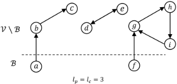
We use the example in Figure 1 illustrate semi-feasible path-cycle packings. Let P1 = abc, P2 = fgh, P3 = igh, C1 = ded, and C2 = ghig. Since lp = lc = 3, we know that P1, P2, C1, and C2 are all feasible. Then the path-cycle packing D1 = {P1, C1, P2} is both semi-feasible and feasible. The path-cycle packing D2 = {P1}∪{C1}∪{P3} is not a feasible packing since P3 is not feasible. However, D2 is a semi-feasible path-cycle packing since P3 is of length ≤ lc and V (P3) ∩ B = ∅.
3.2 ADynamic Programming Algorithm
In this section, we are going to use a dynamic programming method to solve KEP with lp < t and lc < t in O∗ (2n )
| Semi-feasible Packing D = P ∪ C ∪ {D} | Vertex Subset V (D) | |||
|---|---|---|---|---|
| P | C | D | ||
| V (D) ∈ F ab 1,1 | ∅ | ∅ | ab | {a, b} |
| V (D) ∈ F ac 2,2 | ∅ | ∅ | abc | {a, b, c} |
| V (D) ∈ F de 3,1 | {abc} | ∅ | de | {a, b, c, d, e} |
| V (D) ∈ F ed 3,1 | {abc} | ∅ | ed | |
| V (D) ∈ F fg 3,1 | {abc} | ∅ | fg | {a, b, c, f, g} |
| ∅ | {ded} | fg | {d, e, f, g} | |
| V (D) ∈ F dd 4,2 | {abc} | ∅ | ded | {a, b, c, d, e} |
| V (D) ∈ F fg 5,1 | {abc} | {ded} | fg | {a, b, c, d, e, f, g} |
time. This running time bound is not new. Previously, [Xiao and Wang, 2018] showed that KEP can be solved in the same running time bound by using subset convolution. However, their approach cannot combine the representative set method to get the result in this paper. Next, we prove the following theorem.
Theorem 2. There is a dynamic programming algorithm that can deterministically solve KEP with lp < t and lc < t in O∗ (2n ) time.
We use KEPalg to denote the dynamic programming algorithm in Theorem 2. We also recall the assumption that lp < t and lc < t. Under this assumption, we have the following property to bound the length of a feasible path-cycle packing.
Lemma 3. Assume that lp < t and lc < t. A KEP instance (G,B, lp, lc, t) is a yes-instance if and only if there exists a feasible path-cycle packing D such that t ≤ c(D) ≤ 2t.
Proof. If there is a feasible path-cycle packing D such that t ≤ c(D) ≤ 2t, then the instance is a yes-instance by the definition of the problem.
Now we prove the other direction. If (G,B, lp, lc, t) is a yes-instance, then there exists a feasible cycle-path packing D such that c(D) ≥ t. We assume that D is the packing with the minimum c(D) satisfying the above requirement. We are done if it also holds that c(D) ≤ 2t. Otherwise, we have that c(D) > 2t. Since lc < t and lp < t, it holds that c(D) < t for any path or cycle D ∈ D. Let D′ = D \ D. since c(D′ ) = c(D) - c(D) ≥ t, we obtain a new feasible pathcycle packing D′ such that t ≤ c(D′ ) < c(D), which is a contradiction to the minimality of D. So, we know that it holds t ≤ c(D) ≤ 2t.
This lemma says that there exists a path-cycle packing of length at most 2t if the input is a yes-instance. In the process of our dynamic programming, we will compute the vertex subsets of all possible semi-feasible packings with length at most 2t. Finally, we answer the instance by checking whether there is a feasible path-cycle packing of length at least t among all semi-feasible packings we compute.
We can see that a semi-feasible path-cycle packing D = P ∪ C ∪ {D} is feasible if and only if D is a feasible path or cycle. To obtain the ultimate path-cycle packing, we will extend the packing by either increasing the length of the path D by 1 or moving D into P ∪ C and setting a new edge as D. This operation varies depending on the element D. If D is a path (but not a feasible path), we will add one edge to it such that it will either become a feasible cycle or a longer path. If D is a feasible cycle, we move D to C and take a new edge (disjoint with any element in D) as D. If D is a feasible path, we can either increase the length of D by adding an edge at its end or move D to P and take a new edge (disjoint with any element in D) as D.
For a semi-feasible packing D = P ∪ C ∪ D, let V (D) = V (P) ∪ V (C) ∪ V (D). Let Dvu l denote a path from v to u of length l if v ̸= u and a cycle containing v of length l if u = v. We define
Table 1 provides some illustrations of F vu k,l for the example in Figure 1. Our dynamic programming algorithm indeed stores the vertex sets of all possible semi-feasible path-cycle packings by computing F vu k,l for all 1 ≤ k ≤ 2t, v ∈ V , u ∈ V \B and 1 ≤ l ≤ max(lp, lc). The following Lemma 4 says that we can solve KEP by checking F vu k,l .
Lemma 4. A KEP instance (G,B, lp, lc, t) with lp, lc < t is a yes-instance if and only if there exists a tuple (k, v, u, l) such that t ≤ k ≤ 2t, F vu k,l ̸= ∅, and one of the following two conditions holds:
- v ∈ B, u ∈ V \ B and l ≤ lp;
- v = u ∈ V \ B and l ≤ lc.
Proof. We first prove the forward direction. By Lemma 3, we know that if (G,B, lp, lc, t) is a yes-instance, there must be a feasible path-cycle packing D such that t ≤ c(D) ≤ 2t. Since feasible path-cycle packing is also semi-feasible, we know that there exists F vu k,l satisfying the above conditions that contains V (D).
We consider the other direction. Now we have D = (P, C, Dvu l ) with c(D) ≥ t. Since it satisfies the above conditions, we know that Dvu l is actually a feasible path or cycle. Thus D is a feasible path-cycle packing with c(D) ≥ t, which means (G, B, lp, lc, t) is a yes-instance.
We have the following Lemma 5 to compute F vu k,l .
Lemma 5. There exists a dynamic programming algorithm that can compute F vu k,l for all 1 ≤ k ≤ 2t, v ∈ V , u ∈ V \ B and l ≤ max(lc, lp) in time O∗ (2n ).
Proof. Recall that our algorithm is a dynamic programming algorithm. We show how to compute F vu k,l for different values of k, l, v and u by either setting an initial value or giving a transition equation.
We distinguish five cases. In fact, if it is not of the first four cases, then there is no packing satisfying the condition of F vu k,l and we will simply let F vu k,l = ∅. This is Case (v).
If D = {P, C, Dvu 1 } is a semi-feasible path-cycle packing in F vu 1,1 , we know that P = C = ∅. Notice that v ̸= u since there are no self-loops in G and (v, u) ∈ G. The only possible set in F vu 1,1 is {v, u}. Therefore, we let F vu 1,1 = {{v, u}}.
Case (ii): k > l = 1, and (v, u) ∈ A(G).
In this case, for any semi-feasible packing D = {P, C, Dvu 1 } such that V (D) ∈ F vu k,1 , it holds that P ∪ C ̸= ∅ since k > l. We assume that Dv′ u′ l′ is an arbitrary feasible path or cycle in P ∪ C (let v′ = u′ if Dv′ u′ l′ is a cycle, otherwise v′ ̸= u′ ). Then the vertex subset of D′ = {P \ {Dv′ u′ l′ }, C \ {Dv′ u′ l′ },Dv′ u′ l′ } must be contained in F v′ u′ k-1,l′ . Notice that v ̸= u since l = 1. Thus, we can compute F vu k,1 by enumerating all possible v′ , u′ and l′ :
Case (iii): k ≥ l > 1, v ̸= u, l ≤ lp if v ∈ B, and l ≤ lc if v /∈ B.
In this case, for any semi-feasible packing D = {P, C, Dvu l } such that V (D) ∈ F vu k,l , we have that Dvu l is a path of length at least 2 if v ̸= u or a cycle if v = u. Let w be the predecessor vertex of u and Dvw l-1 be the path obtained by removing vertex u from Dvu l . Then the vertex subset of the semi-feasible packing D′ = {P, C, Dvw l-1 } must be contained in F vw k-1,l-1 . Thus, we can compute F vu k,l by enumerating all possible predecessor vertices w:
This case is similar to Case (iii) and we also handle it by enumerating all possible predecessors of vertices v:
Case (v): None of the above four cases holds. It is easy to verify that there is no corresponding packing satisfying the condition. We simply let F vu k,l = ∅.
Next, we analyze the running time bound of the algorithm. Note that our running time bound is not directly obtained by evaluating the number of F vu k,l and the time to compute each F vu k,l . We need a refined analysis. Note that each vertex subset in some F vu k,l can be computed in polynomial time. We only need to evaluate how many vertex subsets are contained in F vu k,l . Let num(k, l, v, u) denote the number of vertex subsets in F vu k,l for values of k, l, v and u. We have that
The number of vertex subsets is bounded by O∗ (2n ) and the running time of the algorithm is bounded by O∗ (2n ).
Now we are ready to prove Theorem 2.
Proof. (of Theorem 2). We prove Theorem 2 by showing that KEPalg can determine where there exists a feasible pathcycle packing of length at least t in time O∗ (2n ).
There are two mains parts in KEPalg. In the first part, we compute F vu k,l for all 1 ≤ k ≤ 2t, 1 ≤ l ≤ max(lp, lc), v ∈ V and u ∈ V \ B. By Lemma 5, we know that the computation can be done in time O∗ (2n ). In the second part, we answer the instance by checking F vu k,l . If there exists a tuple (k, l, v, u) such that F vu k,l is nonempty and either the two conditions in Lemma 4 holds, the answer of the instance is yes. The checking can be done without using more time than part 1.
The algorithm only answer the decision version of the problem. It can also output the corresponding feasible pathcycle packing by adding an additional data structure to store the corresponding path-cycle packings at each state.
3.3 Representative Sets for Kidney Exchange
In this Section, our goal is to obtain a fast algorithm based on KEPalg in Theorem 2. The fast algorithm in this subsection is denoted by KEPalg-rep.
Observe that the exponential factor of the time complexity of KEPalg comes from the cardinality of F vu k,l . Since each collection F vu k,l might contain at most (nk) vertex subsets, the time complexity would roughly be
Notice that we already bound the length of feasible pathcycle packings of KEP in Lemma 3. However, the cardinality of F vu k,l can only be bounded by (nk), which is not tight for our analysis above. This motivates us that we can improve the time complexity by compressing F vu k,l , which might give us a time complexity bounded by t. For example, if we can compress F vu k,l to make it contain at most (2t k ) subsets, then the time complexity would be reduced to ∑2t k=1 (2t k ) = O(4t ).
To compress F vu k,l , our main technique is the efficient computation of representative sets in [Fomin et al., 2016]. We first slightly modify the definition of states in our dynamic programming. Recall that Dvu l denote a path from v to u of length l if v ̸= u and a cycle containing v of length l if u = v. At each state, We define a p-family F vu k,l,p = {V (D) | D = P ∪ C ∪ Dvu l ∧ c(D) = k ∧ |V (D)| = p}. Note that we can compute F vu k,l,p for 1 ≤ k, p ≤ 2t similar to the computation of F vu k,l in Lemma 5.
Let q = 2t - p and ˆ F vu k,l,p denote a q-representative set of F vu k,l,p . In our refined algorithmKEPalg-rep, we want to compute ˆ F vu k,l,p for 1 ≤ k, p ≤ 2t. For the convenience, we use another p-family N vu k,l,p as an intermediate variable to compute ˆ F vu k,l,p . To compute ˆ F vu k,l,p , we first compute N vu k,l,p by following the equation similar to Lemma 5 and then compute ˆ F vu k,l,p ⊆2t-p rep N vu k,l,p by Lemma 2.
We recall the five cases in the proof of Lemma 5 and give the initialization and transition equation of N vu k,l,p and ˆ F vu k,l,p directly as follows:
The following Lemma 6 says that the computation in Equations (4) and (5) gives us a correct representative set of F vu k,l,p .
Proof. We recall that the representative relation is transitive by Lemma 1. By Equation 4, we know that ˆ F vu k,l,p ⊆2t-p rep N vu k,l,p . If it holds that N vu k,l,p ⊆2t-p rep F vu k,l,p , then we are done because ˆ F vu k,l,p ⊆2t-p rep N vu k,l,p ⊆2t-p rep F vu k,l,p . Therefore, we only need to prove that N vu k,l,p ⊆2t-p rep F vu k,l,p .
We prove N vu k,l,p ⊆2t-p rep F vu k,l,p by induction.
For k = 1, by the initialization equation, it holds that N vu k,l,p = F vu k,l,p and N vu k,l,p ⊆2t-p rep F vu k,l,p .
By induction, we assume that
Next, we prove that N vu k,l,p ⊆2t-p rep F vu k,l,p .
Without loss of generality, we take Case (iii) as an example and other cases can be handled similarly. For any vertex subset X ∈ F vu k,l,p in Case (iii), there must be some family F vw k-1,l-1,p-1 containing X \ {u}.
Suppose that Y is disjoint with X and |Y | ≤ 2t - p. Then Y ∪{u} is disjoint with X \ {u} and |Y ∪{u}| ≤ 2t-p+1. By the induction, we have that
Thus, there must be a vertex subset ˆX ∈ ˆ F vw k-1,l-1,p-1 such that ˆX is disjoint with Y ∪{u}. By Equation 5, we know that ˆX ∪ {u} ∈ N vu k,l,p . Let ˆX′ = ˆX ∪ {u}. Since ˆX is disjoint with Y , we have that for any X ∈ F vu k,l,p , if |X ∩ Y | = ∅ and |Y | ≤ 2t - p, then there exists ˆX′ ∈ N vu k,l,p such that | ˆX′ ∩ Y | = ∅.
Therefore, we have proven that N vu k,l,p ⊆2t-p rep F vu k,l,p .
The following Lemma 7 indicates that we can solve KEP by checking ˆ F vu k,l,p .
Lemma 7. Suppose that we are given a KEP instance (G,B, lp, lc, t). If lp, lc < t, then (G,B, lp, lc, t) is a yesinstance if and only if there exists a tuple (k, l, p, v, u) such that ˆ F vu k,l,p ̸= ∅ and either of the two conditions holds:
- t ≤ k ≤ p ≤ 2t, v ∈ B, u ∈ V \ B and l ≤ lp,
- t ≤ k ≤ p ≤ 2t, v = u ∈ V \ B and l ≤ lc.
Proof. The proof is based on the proof of Lemma 4. We first prove the backward direction. By the definition, we have
This implies that if ˆ F vu k,l,p ̸= ∅, then F vu k,l ̸= ∅. Note that if a tuple (k, l, p, v, u) satisfies either the conditions in Lemma 7, then the tuple (k, l, v, u) will naturally satisfies either the conditions in Lemma 4. Thus by Lemma 4, we have that (G, B, lp, lc, t) is a yes-instance.
Next, we consider the forward direction.
Suppose that (G, B, lp, lc, t) is a yes-instance. There exists a vertex subset with the smallest size p0 in all F vu k,l satisfying either the two conditions in Lemma 4. We assume that X0 ∈ F v0u0 k0,l0 without loss of generality. Since X ∈ F v0u0 k0,l0,p0 , we have that ˆ F v0u0 k0,l0,p0 ̸= ∅ by the definition of representative sets. Then it is enough to prove that t ≤ p0 ≤ 2t. Note that p0 ≥ k0 ≥ t. Thus we only need to prove that p0 ≤ 2t.
Let D0 be the corresponding semi-feasible path-cycle packing of X0. If there are only cycles in D0, we have that p0 = k0 ≤ 2t. Otherwise, we can assume that there exists a path P in D0. Since there are no isolated vertices in D0, it holds that p0 ≤ 2k0. If k0 = t, we have that p0 ≤ 2k0 = 2t. Thus, we only need to consider the case k0 > t.
We construct another semi-feasible path-cycle packing D′ by removing the endpoint of P (If P is a path of length 2, we remove it from D directly). Without loss of generality, we assume that V (D′ ) ∈ F v′ u′ k′ ,l′ . Note that we have k′ = k0 - 1 ≥ t. The tuple (k′ , l′ , v′ , u′ ) with F v′ u′ k′ ,l′ ̸= ∅ satisfies either the two conditions in Lemma 4. However, we have that |V (D′ )| < |X0|, which is a contradiction to the minimality of X0. So, we know that it holds p0 ≤ 2t.
We use the following Lemma 8 to compute F vu k,l .
Lemma 8. There exists a dynamic programming algorithm that can compute N vu k,l,p and ˆ F vu k,l,p for all 1 ≤ k ≤ p ≤ 2t, v ∈ V , u ∈ V \ B and l ≤ max(lc, lp) in O∗ (6.855t ) time.
Proof. First, notice that the bottleneck of the time complexity in Lemma 8 is the computation of ˆ F vu k,l,p , i.e., the computation of the representative set of N vu k,l,p by Lemma 2. Let
By Lemma 2, we have that | ˆ F vu k,l,p | ≤ sp,q.
We set x = p p+2q . To simplify our analysis, we first prove the following purely computational result
Note that (1 + 1t )t < e for all t > 0. We have that
Thus, we get (6).
By Equation (5), we have that
By Lemma 2, the time of computing all ˆ F vu k,l,p can be bounded as follows:
We can assume that p = αt (α ∈ (0, 2)) and get
To obtain the time complexity, our goal is to optimize function f (α) = ( 4-α α )α( 4-α 4-2α )4-2α when 0 < α < 2. By direct calculation, we know that f(α) get the maximum value when α0 = 2 - 25 √5 and f(α0) < 6.855. Therefore, we can compute N vu k,l,p and ˆ F vu k,l,p in time O∗ (6.855t ).
Finally, we are ready to prove Theorem 1.
Proof. [Proof of Theorem1] We prove Theorem 1 by showing that the algorithm KEPALG-REP can determine whether there exists a feasible path-cycle packing of total length at least t in time O∗ (6.855t ). The algorithm KEPALG-REP consists of three main components:
Part 1: Handling Large Paths or Cycles. We first check whether lc ≥ t or lp ≥ t. In this case, if there exists a feasible cycle (resp., path) of length at least t when lc ≥ t (resp., lp ≥ t), we return YES and output the corresponding cycle or path. Otherwise, we safely set lc = min(lc, t - 1) and lp = min(lp, t-1). To compute the feasible paths and cycles, we use the algorithm from [Fomin et al., 2016], which runs in time O∗ (6.75t+o(t) ).
Part 2: Computing Table Entries. Next, we compute the sets N vu k,ℓ,p and ˆ F vu k,ℓ,p for all 1 ≤ k ≤ p ≤ 2t, 1 ≤ ℓ ≤ max(lp, lc), v ∈ V , and u ∈ V \ B. According to Lemma 8, this step can be carried out in time O∗ (6.855t ).
Part 3: Answering the Instance. Finally, we determine whether the instance is YES by inspecting the entries ˆ F vu k,ℓ,p . If there exists a tuple (k, ℓ, p, v, u) such that ˆ F vu k,ℓ,p is nonempty and at least one of the two conditions in Lemma 7 holds, we return YES; otherwise, we return NO. This check can be performed within the same time bounds as Part 2.
Similar to KEPALG, the algorithm KEPALG-REP can be extended to output a corresponding feasible path-cycle packing by maintaining an additional data structure during the computation.
4 Conclusion and Discussion
In this paper, we study KEP parameterized by the number of covered recipients t and present a deterministic algorithm with running time O∗ (6.855t ). To achieve this result, we introduce the technique of representative sets into KEP. With modifications to the dynamic programming framework, our approach can be extended to various KEP variants [Krivelevich et al., 2007; Bir´o et al., 2009] as well as to other pathand cycle-related packing problems.
Several promising directions remain for further improving our algorithm. At present, our procedure computes vertex subsets for all semi-feasible path-cycle packings of length at most 2t, as described in Lemmas 3 and 4. It may be possible to optimize this step by focusing solely on vertex subsets of semi-feasible packings of length at most t and then determining in polynomial time whether these can be extended to a full feasible path-cycle packing.
In the realm of randomized algorithms, the best known running time is O∗ (4t ). By applying Lemma 3, one can show that the randomized algorithm of Maiti and Dey [Maiti and Dey, 2022] also achieves a running time of O∗ (4t ). Whether this bound can be further improved remains an open and challenging problem.
Another intriguing avenue for future work is the development of even faster algorithms for KEP when lp and lc are small constants. This consideration is particularly significant in practical applications, where these parameters are often naturally limited in size.
Acknowledgments
We thank the anonymous reviewers for their valuable comments and suggestions that helped improve the quality of this paper. The work is supported by the National Natural Science Foundation of China, under the grants 62372095 and 62502078.
@inproceedings{ijcai2026p262,
  title     = {A Faster Deterministic Algorithm for Kidney Exchange via Representative Set},
  author    = {Tian, Kangyi and Xiao, Mingyu},
  booktitle = {Proceedings of the Thirty-Fifth International Joint Conference on
               Artificial Intelligence, {IJCAI-26}},
  publisher = {International Joint Conferences on Artificial Intelligence Organization},
  editor    = {Diego Calvanese},
  pages     = {2355--2363},
  year      = {2026},
  month     = {8},
  note      = {Main Track},
  doi       = {10.24963/ijcai.2026/262},
  url       = {https://doi.org/10.24963/ijcai.2026/262},
}
TY - CPAPER TI - A Faster Deterministic Algorithm for Kidney Exchange via Representative Set AU - Tian, Kangyi AU - Xiao, Mingyu T2 - Proceedings of the Thirty-Fifth International Joint Conference on Artificial Intelligence, IJCAI-26 PB - International Joint Conferences on Artificial Intelligence Organization PY - 2026 SP - 2355 EP - 2363 DO - 10.24963/ijcai.2026/262 UR - https://doi.org/10.24963/ijcai.2026/262 ER -Copied
Machine-readable versions of this paper, for tools and AI agents:





