BIP Revisited: Enabling Efficient Dominance Pruning for Distributed Constraint Optimization

1 Introduction

Distributed Constraint Optimization Problems (DCOPs) [Hirayama and Yokoo, 1997; Fioretto et al., 2018] provide a foundational modeling framework for cooperative multiagent systems with wide-ranging applications in areas such as sensor networks [Farinelli et al., 2014], scheduling [Pertzovsky et al., 2024] and smart grid [Fioretto et al., 2017].

DCOP algorithms are broadly classified as incomplete or complete. Incomplete algorithms [Maheswaran et al., 2006; Farinelli et al., 2008; Ottens et al., 2017; Nguyen et al., 2019;

∗Corresponding author

Cohen et al., 2020; Deng et al., 2025] find good solutions efficiently, sacrificing optimality. Complete algorithms, in contrast, guarantee optimality through systematic inference or search. Inference-based complete algorithms like DPOP [Petcu and Faltings, 2005] and Action-GDL [Vinyals et al., 2009] utilize dynamic programming to solve a DCOP optimally but require linear messages of exponential size. To address this limitation, subsequent improvements such as MB-DPOP and its variant [Petcu and Faltings, 2007; Chen et al., 2020b] apply cycle-cutting techniques to partition messages into smaller components. Similarly, DPOP with function filtering [Brito and Meseguer, 2010] enhances efficiency by pruning suboptimal tuples through iterative refinement of cost bounds via agent communication.

Alternatively, search-based complete algorithms perform distributed backtracking with linear message sizes but exponential message counts. They rely on bound-dependent pruning, where lower bounds are tightened via communication to prune suboptimal regions. Numerous approaches have been developed to strengthen these bounds: BnB-ADOPT+- AC/FDAC [Gutierrez and Meseguer, 2010] collects projected costs via multi-level arc consistency operations; PT-FB[Litov and Meisels, 2017] employs forward bounding, where agents communicate with unassigned neighbors to obtain bound estimates; ADOPT-BDP[Atlas et al., 2008], DJAO [Kim and Lesser, 2014] and PT-ISABB [Deng et al., 2019] utilize preprocessing inference to collect utility information; and subsequently, HS-CAI [Chen et al., 2020a] further tightens bounds through iterative context-based inference. While these approaches improve pruning effectiveness, their reliance on iterative bound refinement necessitates substantial information exchange among agents, resulting in significant communication and coordination overhead.

To transcend these limitations, a distinct pruning paradigm has emerged. Bound-Independent Pruning (BIP) [Liu et al., 2021] bypasses the reliance on dynamic bound propagation by exploiting intrinsic dominance relationships derived from local constraints. This approach enables agents to identify and prune provably suboptimal regions using only their local knowledge, while maintaining completeness guarantees. However, BIP requires the explicit construction of a contextdependent dominating space through joint optimization over all local constraints, incurring exponential computational and storage complexity.

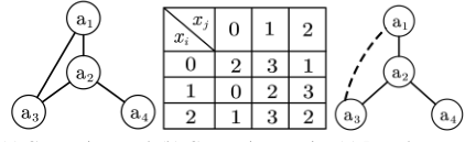
Figure 1: An example of a DCOP and its pseudo tree

To address this challenge, we propose DR-BIP (Decoupled Reformulation of BIP), a novel and sound approach that enables efficient dominance pruning without constructing the dominating space. Our key contributions are: (1) we reformulate dominated-subspace detection into a set of pairwise dominance tests, decouple them across independent constraints into reusable components, and thereby reduce both computational and storage complexity from exponential to polynomial; (2) we formally prove the soundness of DR-BIP by showing its pruning is a subset of BIP's, ensuring compatibility with the BIP framework and enabling modular integration into state-of-the-art tree-based complete DCOP algorithms; (3) we demonstrate through extensive experiments that DRBIP consistently and significantly outperforms both original methods and BIP-enhanced baselines, reducing both computation and communication overhead across diverse benchmark settings.

2 Background

In this section, we introduce preliminaries: DCOPs, pseudo tree, tree-based complete search algorithms, and BIP.

2.1 Distributed Constraint Optimization Problems

A distributed constraint optimization problem [Modi et al., 2005] can be defined by a tuple ⟨A,X,D, F⟩ where A = {a1, a2, ..., an} is a set of agents, X = {x1, x2, ..., xm} is a set of variables, D = {D1,D2, ...,Dm} is a set of finite and discrete domains and F = {f1, f2, ..., fq} is a set of constraint functions. Each variable xi takes a value from its domain Di and each constraint fi : Di1 × · · ·Dik → R⩾0 specifies a cost for each combination of xi1 , ..., xik . Here, we denote the maximal domain size as dmax = maxxi∈X |Di|.

For the sake of simplicity, we follow the common assumptions that all constraints are binary 1 (i.e., fij : Di ×Dj → R⩾0) and each agent controls only one variable (i.e., n = m). Thus, the term agent and variable can be used interchangeably. An optimal solution to a DCOP is an assignment to all the variables that minimizes the total cost. That is,

A DCOP can be visualized as a constraint graph where the nodes denote agents and the edges denote constraints. Figure 1 (a) gives a DCOP with four variables and four constraints. For simplicity, the domain size of each variable is three and all constraints are identical as shown in Fig. 1(b) where i < j.

1 Non-binary constraints can be converted to binary ones via the dual or hidden variable transformation [Bacchus et al., 2002].

2.2 Pseudo Tree

A pseudo tree is a partial ordered arrangement to a constraint graph and can be generated via depth-first search traversal, where different branches are independent of each other. It categorizes constraints into tree edges and pseudo edges (i.e., non-tree edges), thereby allowing the neighbors of an agent ai to be classified, based on the connecting edge type and relative position, as its parent P(ai), pseudo parents PP(ai), children C(ai) and pseudo children PC(ai). We also denote all its (pseudo) parents as AP (ai) = PP (ai) ∪ {P (ai)}, all its (pseudo) children as CD(ai) = C(ai) ∪ PC(ai). The set of ancestors that constrain ai and its descendants is called the separator Sep(ai) [Petcu and Faltings, 2006]. A sample pseudo tree derived from Fig. 1(a) is shown in Fig. 1(c) where the dashed edge is a pseudo edge.

2.3 Tree-based Complete Search Algorithms

Tree-based complete search algorithms perform a systematic search on a pseudo tree. Specifically, each agent ai traverses the subtree rooted at itself under the running context Contexti (i.e., the assignment to Sep(ai)) and avoids expanding suboptimal subspace by exploiting bounds. Contexti is updated upon receiving a context message from ai's (pseudo) parents. When such an update occurs, ai first computes ancestor-constrained cost ap-costi for each di ∈ Di, to initialize its lower bound estimates:

The search then proceeds in either a synchronous or asynchronous manner. In synchronous algorithms, agents must follow a fixed order: ai and its descendants exhaustively explore the subproblem under Contexti before ai reports its final search results, including bounds, to its parent. In contrast, asynchronous algorithms allow agents to continuously update their assignments based on their local view and to continually report their bounds to their parents.

Upon receiving a search-result message from a child, agent ai updates its own bounds by incorporating the received bounds. These updated bounds are then used to prune suboptimal subspaces. Through this iterative process of bound propagation and refinement, agents collaboratively converge to an optimal solution.

2.4 Bound-Independent Pruning Technique

Bound-Independent Pruning (BIP) accelerates tree-based complete search algorithms by pruning dominated regions of the search space using only local knowledge, without relying on bounds. Given the current context Contexti, agent ai first joins all its local constraints involving descendant agents ac ∈ CD(ai) together with the ancestor-constrained cost based on the context into a single cost table:

where DUi -i = ×ac∈CD(ai)Dc, and d-i|xc denotes the component of d-i corresponding to variable xc.

The dominating space (DS) is then constructed by selecting, for each joint assignment d-i of its descendants, the optimal value for its own variable:

Ties in the selection of d∗i are broken alphabetically. The DS contains at least one assignment that can be extended to an optimal solution for the sub-problem rooted at ai. Its complement, called the Dominated Subspace (DDS) and denoted by DUi \SUi i (where DUi =Di ×DUi -i ), can be pruned without losing completeness.

BIP prunes the DDS through a hierarchical process. First, for each value di ∈ Di, the coarse subspace

is considered. If the whole coarse subspace lies inside the DDS, i.e., DUi ⟨di⟩ ⊆ DUi \ SUi i , di is removed from ai's domain. Formally, the set of such dominated values is:

Next, for each remaining value di ∈ Di \ DVi and for each child ac ∈ C(ai), BIP further examines finer subspaces obtained by also fixing the child's value dc:

If DUi ⟨di,dc⟩ ⊆ DUi \ SUi i , value dc can be pruned when ai takes value di. The prunable child values are:

Child ac removes values in DV c i (di) from its domain whenever the context assigns xi = di. Thus, the domain of agent ai after pruning is:

where DV iP(ai) (·) is the set of prunable values computed by ai's parent and piggy-backed through context messages.

3 Motivation

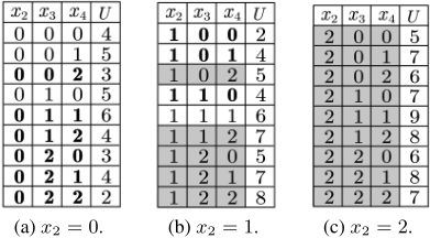
BIP suffers from exponential computational and storage overhead because it must explicitly construct the DS through joint optimization over all local constraints. For instance, consider agent a2 in Fig. 1 with Context2 = {(x1, 1)}. To apply BIP, a2 must first compute SU2 2 by jointly optimizing f12(x1 = 1), f23, and f24 over their shared variable x2. This requires exhaustively enumerating all combinations in U2 (illustrated in Fig. 2, where the elements of SU2 2 are highlighted in bold). Subsequently, a2 derives the dominated subspaces DU2 ⟨x2=2⟩ , DU2 ⟨x2=1,x3=2⟩ , and DU2 ⟨x2=1,x4=2⟩ (shown as gray regions in Fig. 2). Clearly, all local descendant constraints and the context-dependent ancestor cost are computationally coupled through this joint optimization, incurring an exponential computational overhead of O(d|CD(ai)|+1 max ) per context change. Besides, to avoid recomputation upon context changes, BIP precomputes and stores the combination of all local descendant constraints, leading to an exponential storage overhead of O(d|CD(ai)|+1 max ).

The exponential complexity of BIP limits its use in dense, large-scale problems. To mitigate this, BIP introduces a parameter k that restricts its application to agents with |CD(ai)|+1 ≤ k. This restriction, however, severely curtails pruning power. Therefore, we aim to reformulate the identification of dominated subspaces to circumvent the expensive construction of the DS, thereby unleashing the pruning potential of BIP while avoiding exponential overhead.

4 ProposedMethod

In this section, we introduce DR-BIP, a decoupled and sound reformulation for efficiently identifying dominated subspaces in DCOP search. Unlike BIP, DR-BIP directly identifies dominated subspaces through a series of decoupled pairwise dominance tests based on formal dominance properties (defined in Section 4.1). Consequently, the complexity of dominated subspace identification drops from exponential (in BIP) to polynomial.

4.1 Dominance and Conditional Dominance

We begin by formalizing the notion of dominance between values of a variable. Intuitively, a value dominates another if it always yields no worse cost, regardless of how the remaining variables are assigned.

Definition 1 (Dominance). Let Ui be a cost table with scope containing xi, and let di, d′i ∈ Di be two values of xi. Value d′i dominates di with respect to Ui, denoted by d′i ≺Ui di, iff

where DUi -i is the joint domain of all variables in the scope of Ui except xi. If equality holds for some d-i, ties are broken alphabetically in favor of d′i .

A direct consequence of dominance is that the entire subspace corresponding to a dominated value can be pruned.

Property 1. Given a cost table Ui and a value di ∈ Di, if there exists a value d′i ∈ Di such that d′i ≺Ui di, then DUi ⟨di⟩ ⊆DUi \ SUi i .

Proof. For any d = (di, d-i) ∈ DUi ⟨di⟩ , define m = mind∈Di Ui(d, d-i). We have Ui(d′i , d-i) ≤Ui(di, d-i)

from d′i ≺Ui di. If Ui(di, d-i) = m, then Ui(d′i , d-i) = m by the inequality. In this case, d′i precedes di alphabetically and is chosen by tie-breaking. If Ui(di, d-i) > m, di is not a minimizer for d-i. In both cases (di, d-i) /∈ SUi i . Hence DUi ⟨di⟩ ∩ SUi i = ∅, i.e., DUi ⟨di⟩ ⊆DUi \ SUi i .

Property 1 reduces the problem of detecting a (potentially large) dominated subspace to verifying whether a single value di is dominated by some other value d′i . We extend this idea to conditional dominance, where the comparison is restricted to a specific slice of the cost table obtained by fixing a conditional variable xc to a value dc.

Definition 2 (Conditional Dominance). Let Ui be a cost table whose scope includes variables xi and xc. For di, d′i ∈ Di and a fixed value dc ∈ Dc. d′i conditionally dominates di given xc = dc, denoted by d′i ≺Ui(dc) di, iff

where DUi -(i,c) is the joint domain of all variables in the scope of Ui except xi and xc. If equality holds for some d-(i,c), ties are broken alphabetically in favor of d′i .

Analogously, conditional dominance implies that a finer subspace can be pruned.

Property 2. Given a cost table Ui, a value di ∈ Di, and a value dc ∈ Dc of a conditional variable xc, if there exists a value d′i ∈ Di such that d′i ≺Ui(dc) di, then DUi ⟨di,dc⟩ ⊆ DUi \ SUi i .

The proof follows a reasoning analogous to Property 1. Properties 1-2 establish pruning via pairwise dominance. Proposition 1 formalizes the relation to BIP: DR-BIP prunes a subset of BIP's subspaces, ensuring its soundness.

Proposition 1. For any agent ai and context Contexti, DV DR-BIP i ⊆DV BIP i , DV c i (di)DR-BIP ⊆DV c i (di)BIP. Proof. If di ∈ DV DR-BIP i , then by Def. 1 there exists d′i such that d′i ≺Ui di. By Property 1, DUi ⟨di⟩ ⊆ DUi \ SUi i , which by Eq. (3) implies di ∈ DV BIP i . If dc ∈ DV c i (di)DR-BIP, then by Def. 2 there exists d′i such that d′i ≺Ui(dc) di. By Property 2, DUi ⟨di,dc⟩ ⊆ DUi \ SUi i , which by Eq. (4) implies dc ∈ DV c i (di)BIP. Thus both subset relations hold.

Illustrative Example. In Fig. 2, value 0 of x2 dominates value 2 (0 ≺U2 2), which by Property 1 allows the entire subspace DU2 ⟨x2=2⟩ (the left gray columns in Fig. 2(c)) to be pruned; meanwhile, given x3 = 2, value 0 of x2 conditionally dominates value 1 (0 ≺U2(x3=2) 1), which by Property 2 permits the finer subspace DU2 ⟨x2=1,x3=2⟩ (gray cells in the bottom three rows of Fig. 2(b)) to be pruned.

4.2 Decoupled Dominance Evaluation

To efficiently test dominance, we reformulate the pairwise condition as an optimization query. From Def. 1, d′i ≺Ui di holds iff

with alphabetical precedence enforced when the maximum equals zero. The conditional version is:

The key challenge is to evaluate these maximizations without enumerating the exponentially many assignments in DUi -i . We achieve this by exploiting the structure of Ui.

Recall that Ui is defined as the sum of ai's local constraints under the current context (Eq. 1):

Substituting this expression into Eq. (8) yields:

The term ap-costi (d′i ) - ap-costi (di) is independent of d-i and can be pulled out of the maximization. The remaining maximization involves only the static constraints fic. Crucially, each fic depends only on xi and its neighbor xc; there is no coupling among different xc's. Thus, the maximization over the joint domain DUi -i = ×ac∈CD(ai)Dc can be decoupled into independent maximizations over each Dc:

Define the static difference matrix for ac ∈ CD(ai) as

Summing over all descendants gives the aggregated static difference:

∆cd-costi(d′i , di) can be precomputed before search begins and reused throughout the search, because they do not depend on the dynamic context. Only the unary term ap-costi needs to be updated when the context change.

Similarly, for conditional dominance (Eq. (9)), a corresponding derivation for each child ac ∈ C(ai) yields:

where

Again, ∆fic is static and can be precomputed. Thus, evaluating (conditional) dominance reduces to a lookup of precomputed tables plus simple arithmetic operations.

Illustrative Example. Take Fig. 2 as an example. To check if value 2 of x2 is dominated, agent a2 evaluates ∆U2(0, 2) = ∆cd cost2(0, 2) + (ap cost2(0) - ap cost2(2)) = 2 + (-3) = -1 < 0, allowing the entire subspace DU2 ⟨x2=2⟩ to be pruned. To check if value 2 of x3 is prunable when x2 = 1, it computes ∆U 3 2 (0, 1, 2) = ∆U2(0, 1) + ∆f23(0, 1, 2) = 2 + (-4) = -2 < 0, justifying the removal of the finer subspace DU2 ⟨x2=1,x3=2⟩ . Both decisions are made directly via a few table lookups and simple arithmetic operations, without enumerating exponential subspaces.

4.3 Algorithm and Complexity

Algorithm. Algorithm1 outlines the DR-BIP procedure integrated into a tree-based complete search algorithm. Each agent ai executes two phases: a precomputation phase performed once before the search, and a runtime phase triggered whenever the agent's context changes (or when it is the root agent). In the precomputation phase (PRECOMPUTE()), agent ai computes the static table ∆cd costi and for each child ac ∈ C(ai), the table ∆fic (lines 1-2). These tables are context-independent and can be reused throughout the search.

The runtime phase (COMPUTE DVS()) constructs the sets of prunable values: DVi (for agent ai itself) and, for each child ac, DV c i (di). First, ai initializes DVi and all DV c i (di) to empty (lines 3-4). Then, for each value di ∈ Di that has not been pruned by its parent (via DR-BIP) nor by itself (via bound-dependent pruning) (lines 5-6), it calls COMPUTE DV(di) to test whether di is (conditionally) dominated (line 7). COMPUTE DV(di) first builds the set D′i ⊆ Di of candidate dominating values (line 8), then tests dominance by evaluating ∆Ui(d′i , di) for each d′i ∈ D′i (lines 9-10). If a dominating value d′i is found, di is added to DVi and the subroutine returns (lines 11-12). If no dominating value is found, ai proceeds to test conditional dominance through its children. Specifically, for each child ac ∈ C(ai) and its value dc ∈ Dc, it evaluates ∆U c i (d′i , di, dc) for each d′i ∈ D′i (lines 13-16). If a dominating value d′i exists for a given dc, that dc is added to DV c i (di) (line 17).

If after processing a child ac we have DV c i (di) = Dc (line 18), then for every value dc of ac, there exists some (possibly different) value d′i of ai that conditionally dominates di. Consequently, di cannot lead to an optimal solution regardless of how ac is assigned; it is therefore collectively dominated (by potentially different d′i for each dc) and added to DVi (line 19). The evaluation for di terminates (line 20), avoiding redundant checks for the remaining children.

Algorithm 1: Calculating dominated values for ai

Function PR E C O M P U T E(): 1 compute ∆cd costi(d′i , di) by Eq. (13), ∀d′i , di ∈ Di 2 compute ∆fic(d′i , di, dc) by Eq. (16), ∀ac ∈ C(ai), ∀dc ∈ Dc, d′i , di ∈ Di Function COMPUTE DVS(): 3 DVi ← ∅ 4 DV c i (di) ← ∅, ∀di ∈ Di, ac ∈ C(ai) 5 foreach di ∈ Di do 6 if di /∈ DV iP(ai) (Contexti(P(ai))) and di is not pruned by bounds then 7 COMPUTE DV(di) Function COMPUTE DV(di): 8 D′i ←Di \ (DVi ∪ {di}) 9 compute ∆Ui(d′i , di) by Eq. (14), ∀d′i ∈ D′i 10 if ∃d′i ∈ D′i s.t. ∆Ui(d′i , di) ≤ 0 (with tie-breaking) then 11 DVi ← DVi ∪ {di} 12 return 13 foreach ac ∈ C(ai) do 14 foreach dc ∈ Dc do 15 compute ∆U c i (d′i , di, dc) by Eq. (15), ∀d′i ∈ D′i 16 if ∃d′i ∈ D′i s.t. ∆U c i (d′i , di, dc) ≤ 0 (with tie-breaking) then 17 DV c i (di) ←DV c i (di) ∪ {dc} 18 if DV c i (di) =Dc then 19 DVi ← DVi ∪ {di} 20 return

Complexity Analysis. In the precomputation phase, each agent ai constructs two types of static tables. First, it builds the aggregated difference table ∆cd costi of size O(d2max ); each entry ∆fic(d′i , di) for ac ∈ CD(ai) requires maximizing over dmax values of dc, so constructing ∆cd costi takes O(|CD(ai)| · d3max ). Second, for each child ac ∈ C(ai), the agent builds a conditional difference table ∆fic of size O(d3max ), filled in O(d3max ) time via Eq. (16). Hence the total precomputation per agent is O((|CD(ai)| + |C(ai)|) · d3max ).

In the runtime phase, each agent ai computes DVi and DV c i . During context processing, computing DVi involves examining all O(d2max ) value pairs via lookups in ∆Ui. For each child, computing DV c i requires inspecting the O(d3max ) entries of ∆U c i . The overall runtime complexity per agent per context changes is thus O(d2max + |C(ai)| · d3max ).

Memory consumption is dominated by storing ∆cd costi (size O(d2max )) and, for each child, ∆fic (size O(d3max )), leading to total storage O(d2max + |C(ai)| · d3max ).

Discussion. While BIP provides a theoretically powerful pruning mechanism, its exponential complexity in |CD(ai)| + 1 renders it impractical for agents with many children. In practice, BIP is often restricted to agents where |CD(ai)| + 1 ≤ k, limiting its applicability to a small fraction of the search tree. To overcome this fundamental barrier, DR-BIP introduces a fully decoupled and sound reformulation that eliminates the exponential bottleneck entirely. Proposition 1 ensures that DR-BIP's pruning remains sound with respect to BIP. As a result, DR-BIP can be applied to all agents regardless of |CD(ai)|, enabling systematic and scalable pruning across the entire pseudo-tree.

5 Empirical Evaluation

In this section, we first describe the experimental configuration. Then, we compare the DR-BIP-based algorithms with their originals, the corresponding BIP-enhanced versions, and RMB-DPOP [Chen et al., 2020b] on benchmark problems.

5.1 Experimental Configuration

In order to demonstrate its effect on distributed search, DR-BIP is integrated into three state-of-the-art tree-based complete search algorithms: BnB-ADOPT+-FDAC, PTFB, and HS-CAI. Their DR-BIP-enhanced versions are respectively denoted as BnB+DR-BIP, PT-FB+DR-BIP, and HS-CAI+DR-BIP. We compare these DR-BIP-based algorithms with their original counterparts, the corresponding BIP-enhanced versions (i.e., BnB+BIP, PT-FB+BIP, and HS-CAI+BIP), as well as RMB-DPOP-the latest bestperforming algorithm in the DPOP family-on two standard benchmark classes: random DCOPs and scale-free networks. We consider four problem configurations. The first two are random DCOPs with a fixed domain size of 3: a sparse setting with graph density 0.2 and the number of agents ranging from 20 to 30, and a dense setting with density 0.5 and the number of agents from 14 to 24. The third configuration also uses random DCOPs, with 22 agents, density 0.2, and domain sizes varying from 2 to 7. The fourth configuration is based on scale-free networks generated via BA model [Barab´asi and Albert, 1999], with 26 agents, domain size 3, initial clique size m0 = 10, and attachment parameter m1 ranging from 3 to 8. For each configuration, all constraint costs are integers uniformly sampled from [0, 100].

To measure performance, we adopt two metrics: network load (NL), defined as the total volume of information exchanged among agents, and non-concurrent logical operations (NCLOs) [Netzer et al., 2012], which capture hardwareindependent runtime by counting logical accesses to utility and constraint checks. For DR-BIP-enhanced algorithms, the NCLOs counts encompass both the runtime accesses to ∆Ui and ∆U c i and the one-time precomputation of ∆cd costi and ∆fic. For each configuration, we generate 50 random instances and report the average over all successful runs. We set the memory-budget parameter k = 3 for HS-CAI, RMBDPOP, and BIP to match DR-BIP's memory usage for a fair comparison. We also consider BIP with k = 8 to compare DR-BIP against BIP under abundant memory. All experiments ran on an i7-7820X workstation with 32GB of RAM. We enforce a 30-min timeout per algorithm instance.

5.2 Experimental Results

Figure 3 illustrates the performance under varying numbers of agents in the sparse configuration, with the corresponding normalized metrics (NL and NCLOs) presented as percentages relative to the original algorithms in the first two columns of Table 1. Values below 100%, indicating improved performance, are highlighted in bold. Under BIP with k = 3, a clear trend emerges: while the BIP-enhanced algorithms show only marginal improvement or even degradation in some metrics compared to their originals, the DR-BIPenhanced versions consistently and substantially outperform both the original and BIP-enhanced baselines. For instance, the normalized NL and NCLOs of BnB+BIP(k = 3) remain near 100%, whereas BnB+DR-BIP achieves only 15%-33% of the original NL and NCLOs. This pattern holds across PT-FB and HS-CAI, confirming that DR-BIP provides significantly stronger pruning with lower computational overhead than BIP. Furthermore, DR-BIP significantly enhances the scalability of the original algorithms. For instance, while BnB+BIP(k = 3) is limited to problems with at most 24 agents, the DR-BIP-enhanced version of this algorithm scales to 28 agents. Similar scalability gains are observed for PTFB+DR-BIP and HS-CAI+DR-BIP. When BIP is given a larger memory budget (k = 8), its scalability and NL reduction become comparable to those of DR-BIP, and it achieves even lower NCLOs than DR-BIP because more memory is available for caching reusable pruning sets, thereby avoiding redundant computation. Although RMB-DPOP maintains an advantage in NL over most search-based algorithms, it is outperformed in terms of NCLOs by almost all others.

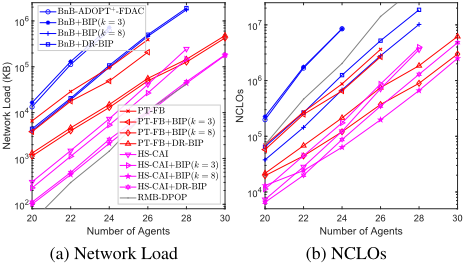
Figure 4 presents the results on dense configurations, with the corresponding normalized metrics shown in the third and fourth columns of Table 1. The BIP-enhanced variants with k = 3 exhibit only marginal improvements over their original counterparts, and in several cases even yield increased NL and NCLOs. In contrast, the DR-BIP-based algorithms maintain a clear advantage, consistently outperforming both the original algorithms and the BIP-enhanced versions across all metrics. However, the performance gaps between DR-BIP and the baselines are narrower than those in sparse settings. This is because denser graphs increase the dimensionality of both coarse and finer subspaces (especially for agents near the root of the pseudo-tree), making the dominance condition stricter and thereby reducing the number of prunable values. BIP-enhanced algorithms with k = 8 achieve NL reduction comparable to their DR-BIP counterparts, but for most algorithms, their NCLOs become substantially higher than those of DR-BIP due to exponential growth in computational cost.

2 BnB+BIP and BnB+DR-BIP yield only one normalized point, as the original succeeds solely on the smallest instance with m1 = 3.

3 All values are normalized against the performance of the corresponding original (unenhanced) algorithms, lower is better.

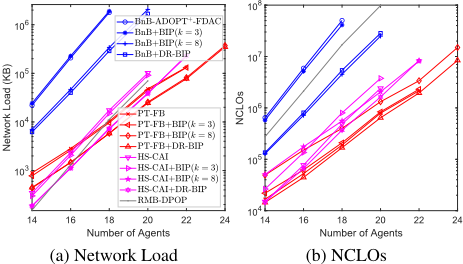
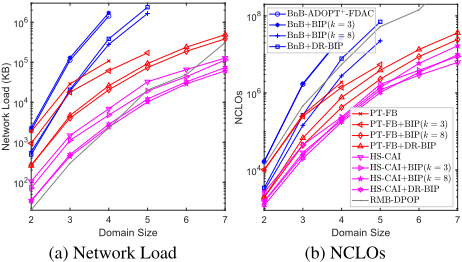
Figure 5 illustrates performance under varying domain sizes. The normalized metrics, given in the fifth and sixth columns of table 1, indicate that DR-BIP remains effective even as domain size grows, though its relative improvement narrows. This reduction occurs because larger domains enlarge both coarse and finer subspaces, which tightens the dominance condition and reduces the number of prunable values. Notably, the BIP-enhanced algorithms (k = 3) struggle with scalability: for example, PT-FB+BIP fails on domains larger than 5, while PT-FB+DR-BIP scales up to domain size 7. Besides, DR-BIP achieves scalability comparable to BIP with k = 8, but with far less memory.

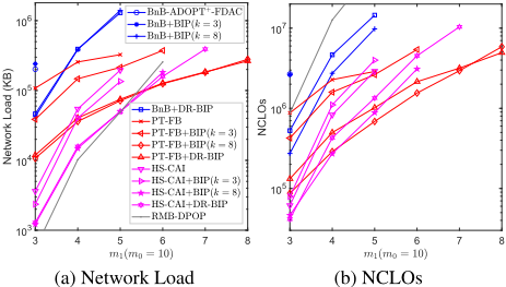
Finally, Fig. 6 presents results on scale-free networks. The corresponding normalized metrics, shown in the seventh and eighth columns of table 1, follow the same trend observed on random DCOPs: the DR-BIP-based algorithms significantly outperform both their originals and the BIP-enhanced versions with k = 3 across all metrics, and their NL reduction is comparable to that of BIP-enhanced versions with k = 8. Moreover, all the DR-BIP-enhanced algorithms scale to larger m1 values than their BIP-enhanced counterparts with k = 3; for HS-CAI, this advantage persists even when BIP is allowed k = 8. These results further evidence the scalability benefits of the decoupled reformulation.

Summary. The experimental results consistently show that BIP with k = 3 provides limited and sometimes inconsistent improvement over the original algorithms, while DR-BIP delivers substantial, robust gains in both efficiency and scalability across diverse benchmark settings. Moreover, even when BIP is granted a much larger memory budget (k = 8), DR-BIP remains highly competitive: it achieves comparable pruning effectiveness (NL) across all problems, while its NCLOs are often lower than BIP's in dense problems. This confirms that DR-BIP retains BIP's core pruning power without its exponential overhead.

6 Conclusion

Building on the foundational principles of boundindependent pruning (BIP) in distributed constraint optimization, we propose DR-BIP, a decoupled reformulation that eliminates the exponential computational and storage complexity barrier of BIP. By decoupling dominated-subspace detection into independent and reusable dominance tests, DR-BIP achieves polynomial complexity while delivering sound and scalable pruning. Our approach is both formally proven and empirically demonstrated to significantly outperform BIP. Beyond DCOPs, the decoupled design of DR-BIP provides a more efficient approach to dominance pruning that can be adapted to other optimization settings where dominance-based reasoning is applicable.

In the future, we will explore extending dominance pruning to dynamic and uncertain DCOP settings, as well as integrating it with learning-based methods to further enhance pruning adaptability and efficiency.