
Compact Modeling in Constraint Programming with Hybrid Tables
Proceedings of the Thirty-Fifth International Joint Conference on Artificial Intelligence. Main Track. Pages 2291-2299.
https://doi.org/10.24963/ijcai.2026/255
© 2026 International Joint Conferences on Artificial Intelligence
Keywords
- Constraint Satisfaction and Optimization: Modeling
- Constraint Satisfaction and Optimization: Constraint optimization problems
- Constraint Satisfaction and Optimization: Constraint satisfaction
- Constraint Satisfaction and Optimization: Constraint programming
Abstract
Hybrid tables, also referred to as `smart' in the literature, represent a valuable modeling technique within Constraint Programming (CP). These tables allow us to handle disjunctive cases (constraining expressions) in a compact and structured way, by authorizing tuples (table entries) to contain simple unary and binary arithmetic restrictions (similar to internal constraints).
In this paper, we show the practical interest of using hybrid tables for planning-like combinatorial puzzles, when the transition from one state to the next can be encoded by a single hybrid table.
Experimental results show that these hybrid models exhibit greater compactness and efficiency in solving compared to their conventional counterparts.
- [Akgün et al., 2025] Özgür Akgün, Ian P. Gent, Christopher Jefferson, Zeynep Kiziltan, Ian Miguel, Peter Nightingale, András Z. Salamon, and Felix Ulrich-Oltean. Tabid: Auto- matic identification and tabulation of subproblems in con- straint models. J. Artif. Intell. Res., 82:1999-2056, 2025.
- [Audemard et al., 2020] Gilles Audemard, Christophe Lecoutre, and Mehdi Maamar. Segmented tables: An efficient modeling tool for constraint reasoning. In Proceedings of ECAI'20, pages 315-322. IOS Press, 2020.
- [Audemard et al., 2023] Gilles Audemard, Christophe Lecoutre, and Charles Prud'Homme. Guiding backtrack search by tracking variables during constraint propagation. In Proceedings of CP'23, pages 9-17, 2023.
- [Barker and Korf, 2012] Joseph Barker and Richard Korf. Solving peg solitaire with bidirectional BFIDA*. In Pro- ceedings of AAAI'12, volume 26, pages 420-426, 2012.
- [Berlekamp et al., 2004] Elwyn R Berlekamp, John H Con- way, and Richard K Guy. Winning ways for your mathe- matical plays, volume 4. AK Peters/CRC Press, 2004.
- [Bessiere et al., 2011] Christian Bessiere, Stéphane Cardon, Romuald Debruyne, and Christophe Lecoutre. Efficient algorithms for singleton arc consistency. Constraints An Int. J., 16(1):25-53, 2011.
- [Boussemart et al., 2016] Frédéric Boussemart, Christophe Lecoutre, and Cédric Piette. XCSP3: an integrated for- mat for benchmarking combinatorial constrained prob- lems. CoRR, abs/1611.03398, 2016.
- [Boussemart et al., 2020] Frédéric Boussemart, Christophe Lecoutre, Gilles Audemard, and Cédric Piette. XCSP3- core: A format for representing constraint satisfaction/op- timization problems. CoRR, abs/2009.00514, 2020.
- [Castro et al., 2022] Margarita P. Castro, André Augusto Ciré, and J. Christopher Beck. Decision diagrams for discrete optimization: A survey of recent advances. IN- FORMS J. Comput., 34(4):2271-2295, 2022.
- [Charlier et al., 2017] Baudouin Le Charlier, Minh Thanh Khong, Christophe Lecoutre, and Yves Deville. Auto- matic synthesis of smart table constraints by abstraction of table constraints. In Proceedings of IJCAI'17, pages 681-687, 2017. IJCAI
- [Debruyne and Bessière, 1997] Romuald Debruyne and Christian Bessière. Some practicable filtering techniques for the constraint satisfaction problem. In Proceedings of IJCAI'97, pages 412-417, 1997. IJCAI
- [Dechter, 2003] Rina Dechter. Constraint processing. Mor- gan Kaufmann, 2003. [Dekker et al., 2017] Jip J. Dekker, Gustav Björdal, Mats Carlsson, Pierre Flener, and Jean-Noël Monette. Auto- tabling for subproblem presolving in minizinc. Con- straints An Int. J., 22(4):512-529, 2017.
- [Frisch et al., 2007] Alan Frisch, Matthew Grum, C. Jeffer- son, B. Martinez Hernandez, and I. Miguel. The design of ESSENCE: A constraint language for specifying combina- torial problems. In Proceedings of IJCAI'07, pages 80-87, 2007. IJCAI
- [Gentzel et al., 2020] Rebecca Gentzel, Laurent Michel, and Willem Jan van Hoeve. HADDOCK: A language and ar- chitecture for decision diagram compilation. In Proceed- ings of CP'20, pages 531-547, 2020.
- [Gharbi et al., 2014] Nebras Gharbi, Fred Hemery, Christophe Lecoutre, and Olivier Roussel. Sliced ta- ble constraints: Combining compression and tabular reduction. In Proceedings of CPAIOR'14, pages 120-135, 2014.
- [Gomes et al., 2000] Carla P. Gomes, Bart Selman, Nuno Crato, and Henry A. Kautz. Heavy-tailed phenomena in satisfiability and constraint satisfaction problems. J. Au- tom. Reason., 24(1/2):67-100, 2000.
- [Hooker, 2012] John N. Hooker. Integrated Methods for Op- timization. Springer, 2012.
- [Jefferson and Nightingale, 2013] Christopher Jefferson and Peter Nightingale. Extending simple tabular reduction with short supports. In Francesca Rossi, editor, Proceed- ings of IJCAI'13, pages 573-579, 2013. IJCAI
- [Jefferson et al., 2006] Christopher Jefferson, Angela Miguel, Ian Miguel, and Armagan Tarim. Modelling and solving english peg solitaire. Computers & Operations Research, 33(10):2935-2959, 2006.
- [Jung and Régin, 2022] Victor Jung and Jean-Charles Ré- gin. Efficient operations between MDDs and constraints. 13292:173-189, 2022.
- [Katsirelos and Walsh, 2007] George Katsirelos and Toby Walsh. A compression algorithm for large arity exten- sional constraints. In Proceedings of CP'07, pages 379- 393, 2007.
- [Lecoutre and Szczepanski, 2020] Christophe Lecoutre and Nicolas Szczepanski. PyCSP3: modeling combinatorial constrained problems in Python. CoRR, abs/2009.00326, 2020.
- [Lecoutre, 2023] Christophe Lecoutre. ACE, a generic con- straint solver. CoRR, abs/2302.05405, 2023.
- [Mairy et al., 2015] Jean Baptiste Mairy, Yves Deville, and Christophe Lecoutre. The smart table constraint. In Pro- ceedings of CPAIOR'15, pages 271-287, 2015.
- [McIlree and McCreesh, 2023] Matthew J. McIlree and Cia- ran McCreesh. Proof logging for smart extensional con- straints. In Proceedings of CP'23, pages 26:1-26:17, 2023.
- Michela Milano and Pascal Van Hentenryck (editors). Hybrid Optimization. Springer, 2011.
- [Milano and Wallace, 2010] Michela Milano and Mark Wal- lace. Integrating operations research in constraint pro- gramming. Ann. Oper. Res., 175(1):37-76, 2010.
- [Nethercote et al., 2007] Nicholas Nethercote, Peter J. Stuckey, Ralph Becket, Sebastian Brand, Gregory J. Duck, and Guido Tack. Minizinc: Towards a standard CP modelling language. In Proceedings of CP'07, pages 529-543, 2007.
- [Ohrimenko et al., 2009] Olga Ohrimenko, Peter J. Stuckey, and Michael Codish. Propagation via lazy clause genera- tion. Constraints An Int. J., 14(3):357-391, 2009.
- [Perron et al., 2023] Laurent Perron, Frédéric Didier, and Steven Gay. The CP-SAT-LP solver. In Proceedings of CP'23, volume 280, pages 3:1-3:2, 2023.
- [Verhaeghe et al., 2017] Hélène Verhaeghe, Christophe Lecoutre, Yves Deville, and Pierre Schaus. Extending compact-table to basic smart tables. In Proceedings of CP'17, pages 297-307, 2017.
- [Wang and Yap, 2023] Ruiwei Wang and Roland H. C. Yap. The expressive power of ad-hoc constraints for modelling CSPs. In Proceedings of AAAI'23, pages 4104-4114, 2023.
- [Zhou and Kjellerstrand, 2016] Neng-Fa Zhou and Håkan Kjellerstrand. The Picat-SAT compiler. In Proceedings of PADL'16, pages 48-62. Springer, 2016.
References were extracted automatically from the PDF and may contain errors.
Full text extracted automatically from the PDF; figures, tables and equations may differ. The PDF is the version of record.
1 Introduction
Constraint Programming (CP) is a technology for tackling hard combinatorial problems. For solving constraint satisfaction/optimization problems, backtrack search remains a central approach, where, at each step, a filtering process (called constraint propagation) is performed in order to reduce the size of the search space (i.e., the domains of the variables). In that context, the search process of a solution (i.e., depth-first exploration) is regularly restarted (in order to avoid the heavy-tailed phenomenon [Gomes et al., 2000]).A "search-based" solver such as ACE [Lecoutre, 2023] remains quite competitive, although some other successful techniques have been deployed in the community, such as integrated approaches [Milano and Wallace, 2010; Milano and (editors), 2011; Hooker, 2012; Perron et al., 2023], lazy clause generation [Ohrimenko et al., 2009; Perron et al., 2023], and decision diagrams [Gentzel et al., 2020; Jung and Régin, 2022; Castro et al., 2022].
Interestingly, a number of modeling languages and libraries have been made available over the years, some of them as free software, such as Essence [Frisch et al., 2007], MiniZinc [Nethercote et al., 2007] and PyCSP3 [Lecoutre and Szczepanski, 2020]. Even when focusing on a limited set of (global) constraints, such as those used in MiniZinc challenges or XCSP3 competitions, it is possible to model a wide range of academic and industrial problems. Indeed, it is well known that global constraints contribute to the success of CP by providing important benefits for both the modeling and the solving phases. This means that such constraints can capture large structural parts of problems (making life easier for users) and usually provide powerful filtering algorithms. Examples of such constraints are AllDifferent, Cardinality, and Cumulative among others.
Another important type of constraint is the one defined from tables. Indeed, it can be applied in any situation (except, of course, when space combinatorial explosion occurs). Initially, such tables were only built from ordinary tuples (composed of integers). Extensions have been proposed over the years with the aim of improving representation and compactness. One can cite compressed tables [Katsirelos and Walsh, 2007], starred tables [Jefferson and Nightingale, 2013], sliced tables [Gharbi et al., 2014], segmented tables [Audemard et al., 2020] and hybrid tables (called smart tables in the original paper) [Mairy et al., 2015]. Interestingly, tuples in hybrid tables can contain simple arithmetic restrictions such as "≥ 2" or "= x1".
So far, published papers on hybrid (smart) tables have discussed how to convert global constraints into hybrid tables [Mairy et al., 2015], introduced dedicated filtering or proof-logging algorithms [Mairy et al., 2015; Verhaeghe et al., 2017; McIlree and McCreesh, 2023], proposed general methods for synthesising hybrid tables [Charlier et al., 2017; Dekker et al., 2017; Akgün et al., 2025], and analysed their expressiveness [Wang and Yap, 2023]. In this paper, we take it a step further, or out of step, by showing how hybrid tables can be useful for modeling and solving problems in a very effective way. We illustrate this advancement by addressing two problems: 1D Rubik's Cube, and Peg Solitaire. For each problem, we present both a conventional modeling approach and a novel approach leveraging hybrid tables. Through comparative analysis, we demonstrate the superior efficiency and effectiveness of solving these problems using hybrid tables.
2 Technical Background
A Constraint Network (CN) is composed of a finite set of variables X, and a finite set of constraints C. Each variable x must be assigned a value from its current domain. Each constraint c is defined by a mathematical relation rel(c) over a sequence of distinct variables, called the scope of c. The arity of a constraint c is the size of its scope. A solution to a CN (X, C) is the assignment of a value to each variable of X such that all constraints of C are satisfied. A classical approach for solving a CN is to perform a depth-first search with backtracking, while filtering domains after each taken decision. The order in which variables are chosen during the depth-first traversal of the search space is decided by a variable ordering heuristic.
A table constraint is a constraint c such that rel(c) is explicitly defined by listing (in a table) the tuples that are allowed (or forbidden) by c. In this paper, a positive (resp., negative) table constraint is written: ⟨x1, x2, . . . , xp⟩ ∈ T (resp., /∈ T) where each xi stands for a variable or a sub-sequence of variables (automatically flattened from a list or matrix of variables) and T stands for a set of tuples. Over the years, there have been many developments about compact forms of tables. Ordinary tables contain ordinary or ground tuples, i.e., classical sequences of values as in (1, 2, 0). Starred tables can additionally contain short tuples [Jefferson and Nightingale, 2013], which are tuples involving the special symbol ∗ as in (0, ∗, 2), and compressed tables can additionally contain compressed tuples [Katsirelos and Walsh, 2007], which are tuples involving sets of values as in (0, {1, 2}, 3). Assuming that the tuples mentioned just above are associated with the sequence of variables ⟨x1, x2, x3⟩, in (0, ∗, 2), x2 can take any value from its domain and in (0, {1, 2}, 3), x2 can take the value 1 or the value 2. Hybrid tables [Mairy et al., 2015] are composed of hybrid tuples, which are tuples containing expressions (called column constraints) of the following forms:
- unary expressions: ∗, <op> v, ∈ S, and /∈ S
- binary expressions: <op> xj and <op> xj + v
with v being a value, S a set of values, and <op> an operator in {<, ≤, =, ̸=, ≥, >}. The hybridization level of a hybrid table is equal to 2 when it contains binary restrictions, 1 otherwise. In terms of expressiveness, one can observe that hybrid tables of level 1 are semantically equivalent to compressed tables. The semantics of hybrid table constraints is simple: an (ordinary) tuple τ is allowed by a hybrid table constraint c iff there exists at least one hybrid tuple η in the table of c such that τ satisfies any component (value or restriction) in η. In order to achieve the property known as Generalized Arc Consistency (GAC) [Dechter, 2003], the filtering algorithm described in [Mairy et al., 2015] assumes no cycle in any constraint graph that can be associated with any hybrid tuple.
About the experiments throughout the paper. For this paper, all models have been developed with PyCSP3 , and all instances have been solved with the constraint solver ACE. Note that i) we are not aware of any other language and/or solver that deals with hybrid tables, and ii) ACE is a competitive solver (implementing efficient propagators for primitive, table and global constraints), as seen in the results of the XCSP3 competitions (www.xcsp.org/competitions). In the next sections, we introduce classical models as well as models based on hybrid tables. For simplicity, we will refer to such models, and instances generated from these models, as C and H, respectively. It is important to note that both PyCSP3 and ACE have the ability of handling hybrid tables. Unless stated otherwise, ACE is run with its default behaviour.
As in [Audemard et al., 2023], for simplicity, the conflictbased variable-ordering heuristics wdeg-cacd, frba/dom and pick/dom will be referred to as wdeg, pick and frba (state-of-the-art generic heuristics due to their robustness). All experiments have been conducted on a computer equipped with XEON CPU 3.5 GHz and 48 GiB of memory. The time limit has been set to one hour per instance, and all times are expressed in seconds.
3 First Case Study: 1DRubik's Cube
The 1D Rubik's Cube is a vector composed of 6 numbers, which can be rotated in 3 different ways in groups of four:
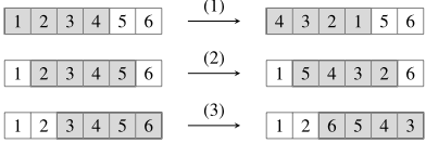
The problem associated with the 1D Rubik's Cube can be defined in general terms: given a scrambled vector V of size n, the objective is to return the shortest sequence of rotations (of length g) so as to restore the original ordered vector. Above, we have n = 6 and g = 4, and the possible rotations are 1, 2, and 3 (as well as 0 for indicating that no rotation is performed). The number r of possible rotations is equal to n - g + 1. A CP model for this problem has been proposed by H. Kjellerstrand (e.g., in Picat [Zhou and Kjellerstrand, 2016]), following a post by O. Kobchenko, and the program proposed by A. Nikitin on his MSX-BASIC page (nsg.upor.net/msx/basic/line.htm).
3.1 Classical Model
For defining a model for this problem, we need to be able to compute the new positions (starting at 1) of the numbers after applying a rotation. This is why we introduce a matrix W defined as follows (for n = 6 and g = 4):
1 2 3 4 5 6 4 3 2 1 5 6 1 5 4 3 2 6 1 2 6 5 4 3Assuming that indexing respectively starts at 0 and 1 for rows and columns, we have for example W1,1 = 4.
Given values for n and g, as well as the authorized horizon (maximal number h of steps) and the initial scrambled vector V , we can define the basic (classical) model, as given in Figure 1 (N∗n stands for {1, . . . , n}.). The variables are defined by statements (8), (9) and (10). We have a two-dimensional array x of variables indicating the status of the vector at each time step. We also need a one-dimensional array y of variables for indicating which rotation is applied at each time step. Finally, a stand-alone variable z indicates the time step when the puzzle is solved.
The first constraints, statements (1) and (2), are about setting the initial and final vectors: in x1, we set the initial scrambled vector, and in xh+1 we set the target ordered vector. We also force rotation 0 (i.e., no rotation) when the problem is solved, by means of a constraint Element; see statement (3). In a second step, two constraint groups are posted
minimize z such that:
Figure 1: Classical Model for the 1D Rubik's Cube
where:
- T1 = {(0, 0)} ∪ {(j, ̸= j) : j ∈ N∗r } is a hybrid table containing r + 1 tuples (of length 2): the ordinary tuple (0, 0) and r hybrid tuples (of level 1);
- T2 = {(∗, . . . , ∗, col(Wj,1), . . . , col(Wj,n), j) : j ∈ Nr} is a hybrid table containing r + 1 tuples (of length 2 × n + 1): each tuple starts with a sequence of n '∗', continues with n expressions of the form col(i) forming 'ci' (in XCSP3 ) where i is computed fromW, and ends with the value j of the rotation (possibly, 0).
Figure 2: Hybrid Model for the 1D Rubik's Cube, obtained from the classical model (in Figure 1) by i) replacing the constraint groups (4) and (5) by the constraint group (11), and ii) replacing the constraint groups (6) and (7) by the constraint group (12)
for breaking some symmetries. Indeed, it is possible to avoid some useless sequences of operations:
- statement (4): if at time t, no operation (0) is performed, then at time t + 1, we can force 0 too;
- statement (5): applying the same operation twice in sequence leaves the vector unchanged.
In a last step, two additional constraint groups implement the main logic of the game: they connect operations with modifications of states. The statement (6) ensures that rotations are properly applied (using the matrix W). The statement (7) ensures that operation 0 leaves the vector unchanged.
3.2 HybridModel
Actually, the last four constraint groups, mentioned above, can be replaced by two groups of hybrid table constraints, as we will show now. The restrictions imposed by the first two constraint groups (out of these last four ones) can be combined in a hybrid table, which gives in format XCSP3 [Boussemart et al., 2016; Boussemart et al., 2020], for our example (n = 6 and g = 4):
The table indicates that 0 can only be followed by 0, that operation 1 cannot be followed by operation 1, and so on.
The two last constraint groups ensure that we pass from a state to another one that is valid (i.e., can be reached). To enforce that, we can instead use a hybrid table involving some binary restrictions. For example, if y1 is set to 0, then we want x1,1 = x2,1, x1,2 = x2,2, . . . By introducing (in XCSP3 ) an expression of the form 'ci' in the jth position of a tuple, we indicate that the variable associated with the ith column must be equal to the variable associated with the jth column. We can then combine all possible transition cases with a single table (note how rotations are managed by the choice of indexes after the symbol 'c'):
The hybrid (variant of the) model for the 1D Rubik's Cube is given in Figure 2. Note how hybrid table constraints are defined by statements (11) and (12).
We have just shown that a model for the 1D Rubik's Cube can be mainly composed of hybrid table constraints: a group of hybrid tables with unary restrictions of the form '̸= i' (hybridization level 1) and a group with binary restrictions of the form '=ci', abbreviated as 'ci' (hybridization level 2).
3.3 Experimental Results
As one can see in Table 1 1 , solving with the solver ACE [Lecoutre, 2023] the most difficult instance hak4(12, 2, 7, 3, 4, 11, 1, 10, 8, 9, 6, 5), mentioned by H. Kjellerstrand on his website (www.hakank.org), gives the following result. The instance built from the hybrid model involves 57 constraints (29 hybrid table constraints, 24 unary constraints, and 4 side constraints) and can be solved in 27 seconds. The instance built from the basic model (i.e., by means of classical intensional constraints) involves 2, 030 constraints (most of them being reified constraints due to complex expressions) and cannot be solved within 1 hour. In Table 1, the number of variables (n), the number of constraints (e) and the time (cpu in seconds) to prove optimality are given. It's worth noting that the use of hybrid tables leads to significantly fewer constraints and variables compared to the classical approach (some decomposition being performed to get primitives). As a result, the time required to solve instances is significantly reduced when using hybrid tables due to their better filtering capabilities: hybrid tables sort of merge (or join) several constraints while guaranteeing a solid level of consistency (GAC).
As the original instances do not seem to be very difficult, we generated a new set of 60 additional instances of this problem: 6 series of 10 instances randomly obtained by varying n from 10 to 15 (while keeping g = 4). Note that we added a group of redundant AllDifferent constraints (on each row of x) because we observed their practical interest for both the classical and hybrid instances. Table 2 highlights the results we obtained, again comparing the behaviour of the solver when instances are generated according to either the basic model or the hybrid one. We also decided to make the comparison on the basis of the three conflict-based heuristics. For each combination (heuristic,model), we give the number (#opt) of solved instances (optimum found and proved), the number (#sat) of instances for which at least a solution was found (but without proof of optimality), and the number (#?) of instances for which no solution was found in one hour. Clearly, the basic model is inefficient compared to the hybrid model. Note that the last column (TT) gives, for a given heuristic, the total time needed to prove optimality on the subset of instances for which both models allowed ACE to prove optimality. This total time is then computed from 8 common instances for wdeg and pick, and 14 for frba. This shows that the hybrid model outperforms the basic model by around two orders of magnitude. Concerning the heuristics, for this problem, one can observe that frba is slightly less effective than wdeg and pick.
1 All models, instances and traces can be downloaded at https: //www.cril.univ-artois.fr/~audemard/traces-ct-ijcai26.zip
| H | C | |||||
|---|---|---|---|---|---|---|
| Instance | n | e | cpu | n | e | cpu |
| hak1 | 145 | 49 | 2 | 825 | 813 | 45 |
| hak2 | 145 | 49 | 2 | 825 | 813 | 55 |
| hak3 | 209 | 57 | 42 | 2,042 | 2,030 | - |
| hak4 | 209 | 57 | 27 | 2,042 | 2,030 | - |
4 Second Case Study: English Peg Solitaire
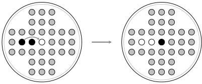
Peg Solitaire is a game (puzzle) played on a board B comprising a number of holes, some of them being occupied by pegs. Any peg can jump over an adjacent peg in order to land in an empty hole, with the jumped-over peg being then removed from the board; see Figure 3. The objective of the game is to make a sequence of moves (jumps), gradually removing the pegs until a goal configuration is obtained. In the English version of the game, the board is in the shape of a cross with 33 holes, as presented in Figure 4. All instances considered in our study will be of a classical nature, commencing with only one hole (at an initial position) and concluding with only one remaining peg (at a final position). Consequently, a sequence of precisely 31 moves must be executed. If the initial and final positions are identical, we are dealing with reversal configurations (instances) of the English Peg Solitaire (EPS), which results in a set of 33 distinct game configurations.
| Heuristic | Model | #opt | #sat | #? | TT |
|---|---|---|---|---|---|
| wdeg | H | 22 | 5 | 33 | 46 5,947 |
| C | 8 | 3 | 49 | ||
| frba | H | 21 | 4 | 35 | 179 |
| C | 14 | 5 | 41 | 10,420 | |
| pick | H | 21 | 7 | 32 | 43 |
| C | 8 | 3 | 49 | 9,215 |

4.1 Classical Model
For this problem, we introduce the set T of possible transitions. There are exactly v = 76 transitions, numbered from 1 to 76. Each transition k ∈ T refers to a list of three pairs of integers representing the positions of the points pk1 , pk2 and pk3 involved in that transition k. We also introduce the (ordered) set P composed of the 33 relevant positions of the board: P = {(1, 3), (1, 4), (1, 5), (2, 3), . . . , (7, 5)}. For any relevant position (i, j) of the board, we suppose that, as in [Jefferson et al., 2006], Changes(i,j) is the set of transitions which change the state of point (i, j), while PegIn(i,j) and PegOut(i,j) are the sets of transitions which place a peg at and remove a peg from point (i, j) respectively.
Given an initial board B (a matrix of size 7×7 where only one peg is absent in a certain relevant position), and considering the fixed horizon h = 31 (since 31 moves must be executed), the basic (classical) model is given in Figure 5. The variables are defined by statements (17) and (18):
- xt,i,j indicates whether, at time t, a peg is present on the board at point (i, j) or not
- yt indicates the number of the move (transition) applied at time t
The first constraints, statement (13), are about setting the initial board in x1. The logic of the game is then implemented
∀t ∈ N∗h , ∀(i, j) ∈ P,
Figure 5: Classical Model for the English Peg Solitaire (EPS)
by statements (14), (15) and (16), indicating when at a certain position (point), nothing changes or a peg appears or disappears.
Note that, here, the final configuration is not imposed (we shall deal with this issue later). When ignoring the trivial unary constraints used to force the initial state, we can find, as mentioned in [Jefferson et al., 2006], that three ternary constraints are posted for each point and each time step, leading to a total of 33 × 31 × 3 = 3, 069 constraints.
4.2 Hybrid (variant of the) Model
It is worth noting that, instead of posting 3, 069 constraints of arity 3 (whose expressions are rather complex), one can post 31 constraints of arity 67. This is made possible by the hybrid nature of the tables we use. The three cases managed separately above can be handled together. By identifying the positions of the three points (p1, p2, p3) involved in each potential move, one can construct a tuple formed by:
- a first sequence of 33 '*' except for the positions of p1, p2 and p3, where we must have 1, 1 and 0 respectively,
- followed by a second sequence of 33 restrictions of the form col(i) (where i is an integer) except for the positions of p1, p2 and p3, where we must have 0, 0 and 1,
- followed by the number of the move (transition).
The first and second parts of the tuple refer to the states of the game at times t and t+1, respectively. Hence, for any point p not involved in the move (i.e., different from p1, p2 and p3), we have '*' in the first part, and 'col(p)' in the second part where 'col(p)' builds 'ci' with i being the index of the point p in P (and so, is the position of the point p in the first part of the tuple). The restrictions imposed by the 'col(p)' expressions ensure that the value of every point on the board that is not involved in the move remains unchanged (let us recall that the operator is implicitly 'equal to'). This results in a table containing exactly 76 tuples, each of which accurately depicts the way the board evolves when a move is performed.
where
Figure 6: Hybrid Model for the EPS, obtained from the classical model (in Figure 5) by replacing the constraint groups (14), (15) and (16) by the constraint group (19)
The hybrid variant of the model is presented in Figure 6. One can observe that the scope of each constraint involves 33 + 33 + 1 variables, corresponding to xt, xt+1 and yt.
The form of the hybrid tables obtained after compilation (i.e., in XCSP3 format) is as follows:
Here, for simplicity, only two tuples are shown: the first one for move 1 (jump towards the right in the first row), and the last one for move 76 (jump towards the left in the last row).
4.3 Symmetry-breaking and Redundant Constraints
Before starting our experimentation, we propose to introduce a number of constraints that we believe will be beneficial. Some of these will be used to break symmetries, while others can be classified as redundant constraints. Concerning symmetry-breaking, although various approaches are possible (for example, exploiting Pagoda functions [Berlekamp et al., 2004; Jefferson et al., 2006; Barker and Korf, 2012], symmetric paths, etc.), we limit ourselves to only two simple mechanisms:
- restricting the choices offered for the first move; by reasoning with the symmetries of the square (horizontal and vertical flips), certain initial moves can be discarded;
- avoiding certain sequences of successive moves: keeping one possible order when transitions are independent, and identifying transitions that cannot be applied one after the other.
Such symmetries are broken by the first two constraint groups, statements (20) and (21), in Figure 7. A transition always has a direction (top, bottom, left, or right). By analysing the first two points p1 and p2 of any transition, one can easily determine its direction. Breaking symmetries of the first move is made possible by posting a unary table constraint (for specific initial positions, a subset of all four directions is identified as symmetry representatives, which is then used to build the table T1). On the one hand, two transitions k and q are independent when they do not share any point: inde(k, q) is true. In this case, if they have to be applied one after the other, they can be applied in any order. This means that we
where:
- T1 is a table (set) restricting the possibilities of the first move (avoiding symmetric first moves);
- T2 = {(k, q) : k ∈ T ∧ q ∈ T ∧ (inde(k, q) ∨ dist(k, q) ≥ 1)}
- T3 = {(k, q) : k ∈ T ∧ q ∈ T ∧ dist(k, q) = 2}
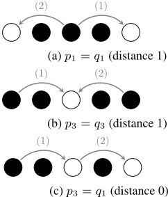
Figure 8: Some illustrations concerning dependent transitions. The first move (1) is composed of points (p1, p2, p3), and the second move (2) is composed of points (q1, q2, q3). When the distance is 1, or more, it means that at least one intermediate move is necessary.
can force transition k to always be applied before transition q to break this form of symmetry (as mentioned in [Jefferson et al., 2006]). On the other hand, some transitions clearly cannot be applied one just after the other. If the distance, dist(k, q), between two transitions k and q is defined as the minimum number of intermediate moves required between them, then a distance of 1 or more implies that we cannot execute them in sequence. An illustration is given in Figure 8. The two observations made above are exploited when computing the table T2 in Figure 7.
It is also possible to strengthen the model (its ability of filtering the search space) by adding some redundant constraints, which correspond to statements (22) and (23) in Figure 7:
- forbidding (with ordinary negative table constraints) the presence of moves that remain incompatible after any intermediate move; the distance between these moves is equal to 2, meaning that at least two intermediate moves are necessary between them. This is the case for a move k with itself (k = q), and for any pair of moves that share pegs as shown in Figure 9 (p1 = q2 and p2 = q1).
where:
- Tz is a table containing tuples of length 34: for each possible final state, the Manhattan distance is computed.
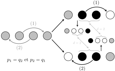
Figure 9: Two transitions at distance 2. Whatever the scenario is, at least two intermediate moves are necessary between them.
- ensuring (with Sum constraints) that we get the right number of pegs at each step; initially, at time t = 1, we have 32 pegs, at time t = 2, we have 31 pegs, and so on.
4.4 Peg Solitaire as an Optimization Problem
Finally, we turn the problem into an optimization problem. The objective is to solve ideally the reversal instances of the Peg Solitaire, meaning that if the initial hole (missing peg) is at position (i, j), then the final remaining peg should be at the same position. To guide the solver towards that ideal position, we compute the Manhattan distance 2 between the initial and final positions by introducing a variable z and posting an ordinary table constraint of arity 34 (the scope is composed of all variables associated with the last state (xh+1) together with the optimization variable z). This table only contains 33 tuples (for each position of the final peg, encoded as a sequence composed of thirty-two 0 and one 1, we associate the corresponding distance). This is shown in Figure 10. Optimality is proved when z becomes equal to 0 (while guaranteeing that all constraints are satisfied).
4.5 Experimental Results
Table 3, which is similar in structure to Table 2, summarizes the first experiment we made with Peg Solitaire. Indeed, we chose to first compare the three main heuristics,
2 This is the distance between two points measured along axes at right angles: if point p1 is at (x1, y1) and point p2 at (x2, y2), the Manhattan distance is |x1 - x2| + |y1 - y2|.
minimize z such that:
| Heuristic | Model | #opt | #sat | #? | TT |
|---|---|---|---|---|---|
| wdeg | H | 28 | 1 | 4 | 6,806 |
| C | 16 | 1 | 16 | 16,284 | |
| frba | H | 32 | 1 | 0 | 8,173 |
| C | 30 | 2 | 1 | 21,606 | |
| pick | H | 24 | 3 | 6 | 6,310 |
| C | 19 | 4 | 10 | 20,374 |
and their effect on both the hybrid and the classical models. The results underline two important points. First, the hybrid method proves to be significantly more effective than the classical one, regardless of the heuristic used: more instances are solved to optimality, and further analysis shows that it is approximately 2.5 times faster on commonly solved instances. Second, frba is a heuristic which is significantly more efficient than wdeg and pick, solving 32 out of 33 instances within 1 hour (against 28 and 24 instances, resp.).
In the light of these results, it was decided to carry out further experiments using only the hybrid model (and the frba heuristic), with the aim of adjusting the strategy of the solver ACE in order to obtain, if possible, some improvements (i.e., speeding up search and/or solving all instances). More specifically, we have tested:
- SAC, the use of Singleton Arc Consistency (SAC) [Debruyne and Bessière, 1997; Bessiere et al., 2011] at preprocessing, because we observed that some additional values can be initially removed by this property;
- PV, the use of values identified as priority; they correspond to transitions that move corner pegs towards the middle (e.g., a transition from (2,0) to (2, 2) as indicated in [Jefferson et al., 2006]), and when no such transition is possible, the solver reverts to the naive ascending order;
- ¬RC, discarding all redundant constraints;
- ¬SB, discarding all symmetry-breaking constraints.
The experimental results obtained with these different strategies are shown in Table 4. The first thing to note is that, when symmetry-breaking is disabled (frba-¬SB), the performance of the solver is severely compromised. As only 20 instances were solved without symmetry-breaking, it was deemed prudent to calculate the total time (TT) for common instances solved by all strategies except this one. Redundant constraints also play an important role in speeding up the search. Disabling them allows the resolution of 28 optima, but 2 instances remain unresolved, and the cumulative time required to solve them becomes very high (11, 993). A second important observation is that SAC is a major performance accelerator, reducing TT by a factor of about 4. On average, about 25 values are specifically deleted by SAC during preprocessing (about 0.8% of all values). Finally, moving the corner pegs towards the centre of the board (PV) is successful because i) when combined with SAC, the total time is the best, and ii) when used alone, it allows all 33 instances to be solved. These results look interesting, compared to those mentioned in [Jefferson et al., 2006] (although it is true that this study is 20 years old). However, it seems that the original bidirectional breadth-first IDA* (BFIDA*) proposed in [Barker and Korf, 2012] remains a formidable competitor for solving such puzzles. Note that we haven't included similar results obtained for the Peg Solitaire variants studied in [Jefferson et al., 2006] due to lack of space. With hybrid tables, the cumulative time to solve all 10 Solitaire Patterns and 7 Fool Solitaire instances (see tables 6 and 7 in [Jefferson et al., 2006]) takes less than 25 minutes.
| #opt | #sat | #? | TT | |
|---|---|---|---|---|
| frba-PV | 33 | 0 | 0 | 7,537 |
| frba | 32 | 1 | 0 | 8,699 |
| frba-SAC-PV | 31 | 2 | 0 | 1,483 |
| frba-SAC | 28 | 5 | 0 | 1,944 |
| frba-¬RC | 28 | 3 | 2 | 11,993 |
| frba-¬SB | 20 | 11 | 2 | - |
5 Conclusion
In this paper, we have shown how hybrid tables can be very effective from both a modeling and a solving perspective. Our first objective was to contribute to the reinforcement of successful mechanisms in CP modeling/solving: here, we have shown that hybrid tables can be useful to a CP solver, compared to classical constraints implemented in the same CP solver. To the best of our knowledge, this is the first paper to address these two aspects using several case studies based (almost) entirely on tables. We insist on the compactness of the hybrid models, drastically reducing the number of constraints while maintaining GAC.
We have shown that for certain planning-like combinatorial puzzles simulating the evolution of a vector (1D Rubik's Cube) or a matrix (Peg Solitaire), the transition from one state to the next can be encoded by a single hybrid table. As a consequence, as such hybrid tables can be seen as the union (join) of several classical constraints, they become more powerful in terms of filtering (just like an AllDifferent is stronger than a clique of binary not-equal constraints). Once two constraints that share at least two variables are combined to form a hybrid table, the filtering ability is very likely to increase (e.g., our hybrid models introduced in this paper achieve speed-ups ranging from a factor of 2 to two orders of magnitude). However, increased model compactness does not automatically yield better performance, as search strategies remain crucial. Some conflict-based heuristics may require adaptation to handle the large arity of hybrid table constraints.
Acknowledgements
This work was supported by State funding managed by the French National Research Agency (ANR) under France 2030 and by the European Union through NextGenerationEU, reference 22-EXES-0009.
@inproceedings{ijcai2026p255,
  title     = {Compact Modeling in Constraint Programming with Hybrid Tables},
  author    = {Lecoutre, Christophe and Samy Modeliar, Mouny and Audemard, Gilles and Paris, Nicolas and Szczepanski, Nicolas},
  booktitle = {Proceedings of the Thirty-Fifth International Joint Conference on
               Artificial Intelligence, {IJCAI-26}},
  publisher = {International Joint Conferences on Artificial Intelligence Organization},
  editor    = {Diego Calvanese},
  pages     = {2291--2299},
  year      = {2026},
  month     = {8},
  note      = {Main Track},
  doi       = {10.24963/ijcai.2026/255},
  url       = {https://doi.org/10.24963/ijcai.2026/255},
}
TY - CPAPER TI - Compact Modeling in Constraint Programming with Hybrid Tables AU - Lecoutre, Christophe AU - Samy Modeliar, Mouny AU - Audemard, Gilles AU - Paris, Nicolas AU - Szczepanski, Nicolas T2 - Proceedings of the Thirty-Fifth International Joint Conference on Artificial Intelligence, IJCAI-26 PB - International Joint Conferences on Artificial Intelligence Organization PY - 2026 SP - 2291 EP - 2299 DO - 10.24963/ijcai.2026/255 UR - https://doi.org/10.24963/ijcai.2026/255 ER -Copied
Machine-readable versions of this paper, for tools and AI agents:





