Rolling in Classical Planning with Conditional Effects and Constraints

1 Introduction

In classical planning, the environment in which agents operate is represented through Boolean variables, and actions are idempotent, i.e., applying the same action once or multiple times results in the same state. The idempotence property falls if we introduce conditional effects (CEs), i.e., actions with state-dependant effects. Dealing with one application of an action with CEs has been extensively studied and two main approaches exist: either (i) one deals with CEs in a native way, i.e., by encapsulating CEs directly in the procedure searching for a plan [Rintanen, 2011; R¨oger et al., 2014; Katz, 2019], or (ii) one compiles-away actions with CEs [Gazen and Knoblock, 1997; Nebel, 2000; Gerevini et al., 2024]. Logic-based native approaches (see, e.g. [Rintanen, 2011]), are all based on planning as satisfiability (PaS) [Kautz and Selman, 1992] where a planning task Π is solved by first encoding Π into a corresponding logic formula Πn incorporating a bound (or number of steps) n, and then searching for a model of Πn, increasing n upon failure. In all existing PaS approaches, an action a can be applied at most once per step, and thus, a plan with r consecutive repetitions of a will be found in a number of steps n ≥ r. The rolling technique, introduced for numeric planning in [Scala et al., 2016], allows modelling consecutive repetitions of a in a single step, thus reducing the bound n. Rolling has proved to be very effective in numeric planning [Scala et al., 2016; Cardellini et al., 2024]. Similarly to the numeric case, constraints on the state-space must be carefully handled while rolling to assure the plan's validity [Scala et al., 2016].

In this paper, we ask if rolling can be effectively exploited also in classical planning with CEs and constraints. Firstly, we show that planning with CEs remains PSPACE-complete [Nebel, 2000] even in the limit case of problems with a single action, and thus, finding how many times the action has to be consecutively applied is a difficult problem on its own. Secondly, we present a PaS encoding in which an action can be consecutively repeated in a single step. Given an action a, we (i) compute its transition relation Ta representing all the states reachable after one application of a, (ii) compute its transitive closure (TC) relation T + a (see, e.g., [Matsunaga et al., 1993]) representing the states reachable after at least one application of a, and (iii) define a PaS encoding Π+, exploiting a propositional variable a+ to denote if action a is applied at least once, and T + a to compute the states reachable with a. Given a model for the encoding Π+ at bound n, we determine the number of times each action a is applied by exploiting the intermediate formulae used to compute T + a .

Since deciding the reachability of a state by repetitions of an action with CEs is PSPACE-complete, the computation of the TC T + a can become impractical. To alleviate this burden, we (i) show how constraints can be leveraged to simplify T + a , and (ii) construct T + a through Reduced Ordered Binary Decision Diagrams (simply BDDs) [Bryant, 1985], which have been widely employed for this purpose in Model Checking [Burch et al., 1992; Clarke et al., 1996] due to its often compact representation and canonicity. If the computation of T + a becomes unpractical even then, we can limit the time on the construction of T + a and exploit the intermediate formulae T m a with m ≥ 0 produced while constructing T + a - in the best case being T m a = T + a and in the worst case being T 0 a = Ta - modelling the states reachable in up to 2m repetitions of a, reducing by a factor of 2m the bound required to find a plan.

We prove that our approach is correct and complete, and run an experimental analysis on novel domains where a plan must have repetitions of an action. The analysis confirms our theoretical results and, by comparing to the case where rolling is disabled, confirms the benefits of rolling.

2 Preliminaries

2.1 Classical PlanningWith CEs and Constraints

A classical planning task with CEs and constraints (in the following, just planning task) is a tuple Π = ⟨V,A, I,G,C⟩. The set V contains propositional variables with domain {⊤,⊥}, the symbols for truth and falsity. The set V induces the set of literals lit(V ) = {v | v ∈ V } ∪ {¬v | v ∈ V }. Let L ⊆ lit(V ), we define L+ = {v | v ∈ L} and L- = {v | ¬v ∈ L}. In the following, we consider only consistent sets L of literals, i.e., with L+ ∩L- = ∅. An action a ∈ A is a pair ⟨pre(a), post(a)⟩ where the precondition pre(a) is a propositional formula over V and the postcondition post(a) is a set of CEs of a. A CE e is a pair ⟨cond(e), eff(e)⟩ where cond(e) is a propositional formula representing the conditions of applying the effects eff(e) ⊆ lit(V ). If v ∈ eff(e) we say that e adds v, if ¬w ∈ eff(e) we say that e deletes w. We denote by add(a) and del(a) the set of variables added or deleted by a, with ∆+a (v) and ∆-a (v) the set of CEs of an action a that adds or deletes a variable v If, for each e ∈ post(a), we have cond(e) = ⊤, then a is without CEs, and with CEs otherwise. If, for each a ∈ A, a is without CEs (resp. with CEs), then also Π is. A state is a set s ⊆ V containing the variables which are true in s, while V \ s are false in s. We denote by S = 2V the set of all states. To conclude the description of Π, we have the initial state I ∈ S, and the goal condition G and the constraints C, both defined as propositional formulae over V . We take for granted the standard notions of satisfiability and write s |= ϕ to mean that state s satisfies the propositional formula ϕ. An action a is applicable in a state s if (i) s |= pre(a), (ii) there exists at least one CE e ∈ post(a) such that s |= cond(e), and (iii) there are no conflicting CEs, i.e., for each v ∈ V , e+ ∈ ∆+a (v) and e- ∈ ∆-a (v) then s ̸|= cond(e+) ∧ cond(e-). Applying an action a in a state s results in a state s′ = res(s, a), such that either

1. s′ is undefined if either s is undefined or a is not applicable in s, or
2. for each v ∈ V we have v ∈ s′ iff either (i) v ∈ s and there is no CE e ∈ ∆-a (v) such that s |= cond(e), or (ii) there is a CE e ∈ ∆+a (v) such that s |= cond(e).

Applying a sequence of n actions α = a1; . . . ; an from a state s0 induces a sequence of n+1 states s0; . . . ; sn where si+1 = res(si, ai+1) with i ∈ [0, n) and we say that sn = res(s0, α). The sequence α is valid if si |= C for each i ∈ [0, n]. A valid plan π for a planning task Π is a valid sequence of actions π = a1; . . . ; an such that res(I, π) |= G. We denote by |π| = n the length of π = a1; . . . ; an, and with ak , with k ≥ 0, the sequence of k repetitions of a.

2.2 Planning as Satisfiability

Let Π = ⟨V,A, I,G,C⟩ be a planning task. In planning as satisfiability (PaS) [Kautz and Selman, 1992], an encoding E of Π is a tuple ΠE = ⟨X,A, I(X), T E (X,A,X ′ ), G(X)⟩ where X is a finite set of state variables, in our case equal to V , A is a finite set of action variables, I(X) is the initial state formula, i.e., the conjunction of {v | v ∈ I} ∪ {¬w | w ∈ V \ I}, and, G(X) is the goal formula, i.e., the formula G.

Each encoding E is characterized by the symbolic transition relation T E (X,A,X ′ ), where X ′ = {v′ | v ∈ X} is the set of next state variables. A model µ for T E is an assignment µ: X ∪A∪ X ′ ↦→ {⊤,⊥}. As standard for PaS encodings, ΠE has to guarantee correctness and completeness. 1

1. Correctness: each model µ of T E corresponds to at least one valid sequence of actions α such that if s = {v | µ(v)} and s′ = {v | µ(v′ )} then s′ = res(s, α).
2. Completeness: for each state s and action a applicable in s, if s′ = res(s, a), s, s′ |= C, then there is a model µ of T E s.t. s = {v | µ(v)}, s′ = {v | µ(v′ )}.

Given ΠE , in the PaS approach, an integer n ≥ 0 called bound or number of steps is fixed, n + 1 disjoint copies X0, . . . ,Xn of the set X of state variables, and n disjoint copies A1, . . . , An of the set A of action variables are made, and the E encoding of Π with bound n is the formula

in which I(X0) is obtained by substituting in I(X ) each variable v ∈ X with v0 ∈ X0 , and similarly for T E and G. The satisfiability of ΠEn is checked by calling a SAT solver starting from n = 0 and incrementing n until a model (and thus a valid plan) is found. The correctness of T E ensures the correctness of ΠE : each model of ΠEn corresponds to a valid plan. The completeness of T E ensures the completeness of ΠE : if there exists a plan for Π of length n, ΠEn is satisfiable.

3 Complexity of Rolling

In this section, we present our main complexity result for classical planning with CEs.

Theorem 1. Deciding whether a valid plan exists for a classical planning task with CEs and with only one action is PSPACE-complete.

Proof. Let Π = ⟨V, {a}, I,G,⊤⟩. (Membership) The problem is in PSPACE because the size of a state is bounded by |V | and we iteratively apply a from I until we reach sn |= G. Since there are at most 2|V | possible states, no more than 2|V | repetitions of a are required to reach sn. (Hardness) Let M be a Deterministic Turing Machine (DTM) with bounded tape, i.e., M = ⟨Q, Σ, Γ, δ, q0, qa, n⟩ (see, e.g., [Sipser, 1997]). Q is the set of states, Σ the input alphabet, Γ the tape alphabet including Σ and the symbol ⊔ for "blank", δ is a partial function δ : Q × Γ ↦→ Q × Γ × {L,R}, the states q0, qa ∈ Q are the initial and accepting states, respectively, n ∈ N is the bounded length of the tape. Let the input of the DTM be y1; . . . ; ym with yi ∈ Σ and m ≤ n. We reduce the DTM M to the planning task Π such that

1 In the rest of the paper µ(v) corresponds to the equation µ(v) = ⊤ and s, s′ |= ϕ to s |= ϕ ∧ s′ |= ϕ.

Where tpi is used to control the allowed cells of the tape, ati,q signals that the DTM is in tape's cell i and state q, and ini,x signals that cell i contains symbol x. The only action in Π is a = ⟨⊤, post(a)⟩ where, for each i ∈ [1, n] and (q, x) ∈ Q × Γ, if δ(q, x) = (q′ , x′ , L) then post(a) contains

i.e., if the DTM is in cell i and state q, reading x, and the cell on the left is allowed, then the DTM moves left to cell i-1 and to state q′ and the symbol in cell i is replaced with x′ . Similarly, if δ(q, x) = (q′ , x′ , R) then post(a) contains

Finally, for each i ∈ [1, n], post(a) contains

i.e., the DTM accepts if it is in the accepting state, and it is not reading any symbol that would change the DTM state.

Since the CEs encode the transition δ, a valid plan can be found iff M accepts. Since |Q| × |Γ| × n is polynomial w.r.t. the size of M, we conclude that a DTM with polynomially bounded tape and its input can be polynomially reduced to a planning task with only one action with CEs.

4 Rolling Actions with Conditional Effects

In this section, we show how to exploit rolling of actions with CEs. Firstly, we describe the concept of transition relation, i.e., a logic formula denoting the states reachable with one application of an action. Then, we show how to compute its transitive closure (TC), obtaining a logic formula denoting all the states reachable by at least one repetition of an action.

4.1 Transition Functions and Transition Relations

Let Π = ⟨V,A, I,G,C⟩ be a planning task. The transition function of a ∈ A is a function Ta : S × S ↦→ {⊤, ⊥} such that, for each s, s′ ∈ S, we have Ta(s, s′ ) = ⊤ iff (i) a is applicable in s and (ii) s′ = res(s, a). Notice how, for now, we allow s, s′ ̸|= C, which we will disallow later on.

As standard for PaS encodings (see, e.g., [Rintanen, 2011]), we model an action's transition function through a transition relation. A transition relation of an action a is a propositional formula Ta(X, X ′ ), where X = V and X ′ = {v′ | v ∈ X} is a copy of X. The models of Ta represent the states s, s′ ∈ S such that Ta(s, s′ ) = ⊤. For the case of classical planning with CEs and constraints, the transition relation Ta(X,X ′ ) is the conjunction of the union of the following sets of formulae:

1. prea which contains

ensuring the preconditions of a and the conditions of at least one CE in post(a) are satisfied,

1. effa(V ) which contains, for each v ∈ V ,

ensuring s′ = res(s, a), i.e., v′ is true if v is true and no condition of a CE deleting v (∆-a (v)) is satisfied, or at least one condition of a CE adding v (∆+a (v)) is satisfied,

1. conflicta(V ), containing for each v ∈ V and for each e1 ∈ ∆+a (v) and e2 ∈ ∆-a (v)

ensuring no conflicting CEs' conditions are satisfied.

4.2 Computing the Transitive Closure

Let Π = ⟨V, A, I, G, C⟩ be a planning task and a be an action of Π with transition function Ta. The TC function of a is T + a : S × S ↦→ {⊤,⊥} such that for each state s, s′ ∈ S, T + a (s, s′ ) = ⊤ iff (i) a is applicable in s, and (ii) there exists a valid sequence ak with k ≥ 1 such that s′ = res(s, ak ).

The TC function T + a can be computed iteratively (see, e.g. [Matsunaga et al., 1993]) using the TC relation T + a , starting from the transition relation Ta. Let T i a (X , X ′ ) be the i-th step transition relation of a, such that T 0 a (X,X ′ ) = Ta(X,X ′ ) and for each i ≥ 0,

where C(X) is obtained by replacing the variables in C with the ones in X (and similarly for X ′ and X ′′ ). The models of T i a represent the states s, s′′ ∈ S such that the i-th step transition function T ia (s, s′′ ) = ⊤. Notice how T i+1 a (s, s′′ ) is true if either s ̸|= C or s′′ ̸|= C. This relaxation allows, in some cases, a more compact formula for T + a , and will be better explained in Section 4.3. The requirement that s, s′′ |= C will be enforced at a later stage.

Continuing the computation, by the finiteness of the states, there exists a p ≥ 0 - called the fix-point index of Ta- such that T p a (X,X ′ ) is logically equivalent to T p+1 a (X,X ′ ). By representing each T i a with BDDs, which are canonical representations of propositional formulae, we check logical equivalence of T p and T p+1 by assessing if they have the same BDD. The TC relation T + a is thus the fix-point relation T p a .

Lemma 1. Let p be the fix-point index of the transition function Ta of an action a of a planning task with constraints C. For each i ∈ [0, p] and s, s′′ ∈ S s.t. s, s′′ |= C

Sketch Proof. For i = 0, T 0 a (s, s′′ ) ↔ Ta(s, s′′ ) which by definition models s′′ = res(s, a), i.e., 20 = 1 repetitions of a. For i > 0, by Eq. 2, T 1 a (s, s′′ ) models the states reachable after up to 2 repetitions of a: we can model (i) s′′ = res(s, a2 ) since T 0 a (s, s′ ) models s′ = res(s, a) and T 0 a (s′ , s′′ ) models s′′ = res(s′ , a), and (ii) we can model s′′ = res(s, a1 ) because T i a (X , X ′′ ) ∧ C(X ) ∧ C(X ′′ ) entails T i+1 a (X,X ′′ ) in Eq. 2. Since s, s′′ |= C, Eq. 2 guarantees that s′ |= C. By induction, we prove that T ia (s, s′′ ) can model up to 2i repetition of a , since we have T i-1 a (s, s′ ) to reach s′ from s in at most 2i-1 steps, and T i-1 a (s′ , s′′ ) to reach s′′ from s′ in at most 2i-1 steps.

The function T ia (s, s′ ) thus specifies if s′ is reachable from s in at most 2i repetitions of a. In the following sections we will also need to know if the state is reachable in exactly 2i repetitions of a. For this reason, we introduce the i-th step exponential reachability relation of a as Ria such that R0a (X , X ′′ ) = Ta(X , X ′′ ) and for i > 0

The i-th step exponential reachability function Ria : S×S ↦→ {⊤, ⊥} can be retrieved from Ria as for T ia .

Lemma 2. Let a be an action and let Ria be its i-th step exponential reachability function.

Sketch Proof. As for Lem. 1, by induction on Eq. 3.

As stated in the introduction, the TC computation can become intractable, due to formulae becoming exponentially long, even when employing BDDs. However, the computation of the TC can be stopped at any time, before its fix-point index p, returning the last computed relation T m a with m ∈ [0, p], which models the states reachable with up to 2m repetitions of a (Lem. 1). We name m the timeout index.

4.3 Transitive Closure and Constraints

Let Π = ⟨V,A, I,G,C⟩ be a planning task. In this section, we show how constraints can, in some cases, simplify TCs.

Example 1. A robot can move in one direction on a ring tape with k cells, where the last and first cell are connected. The problem can be modelled as a planning task where V = {c1, . . . , ck} models the position on the tape, I = {c1}, and there is only one action mv with pre(mv) = ⊤ and

Let's suppose that C = ⊤, i.e., there are no constraints. One would imagine that, since the robot can reach any cell in the ring tape by applying mv at most k times, then the TC function T + mv (s, s′ ) would be ⊤ for each s, s′ ∈ S. However, the TC has to consider also the cases where |s| or |s′ | is not 1, e.g., T + mv ({c1}, {c2, c4}) = ⊥. To avoid this problem, we can specify in C that the robot must be exactly in one cell, i.e.,

Employing this constraint we have that T + mv (s, s′ ) = ⊤ for each s, s′ ∈ S, since, if either s ̸|= C or s′ ̸|= C then, in Eq. 2, the l.h.s. of the implication is ⊥. Intuitively, if the robot starts from any state s0 |= C it can reach any other state sn |= C by passing only in states si |= C, i ∈ (0, n). If the robot starts from a state s ̸|= C then it can reach any state. By guaranteeing that the robot always start moving from a state s |= C (later in the encoding), we will guarantee correctness.

The use of constraints thus can, in some cases, be beneficial in producing smaller T + a by not considering states which do not align with our knowledge of the problem.

5 The Closure-Encoding

Let Π = ⟨V,A, I,G,C⟩ be a planning task. For each action a ∈ A, let Ta(X,X ′ ) be the transition relation of a and let T + a (X,X ′ ) be its TC relation. We now present the closure encoding Π+ for Π. As standard for PaS approaches, the sets X, A, X ′ represent the current state, action, and Algorithm 1 Computation of the rolling of a needed to reach s′′ from s.

1: global T 0 a , . . . , T p a ,R0a , . . . ,Rpa //previously computed 2: function REPETITIONS(a, s, s′′ , p) 3: if T 0 a (s, s′′ ) then 4: return 1 5: for j ∈ [1, p] do 6: if T j a (s, s′′ ) then 7: s′ ← s′ : Rj-1 a (s, s′ ) 8: return 2j-1 + REPETITIONS(a, s′ , s′′ , j - 1) 9: return -1

next state variables. In A there is a propositional variable a+ for each action a in A, denoting if a is repeated at least one time. The current state variables X are equal to V and the set X ′ is a copy of X . The closure-encoding for Π is thus Π+ = ⟨X,A, I(X), T +(X,A,X ′ ), G(X)⟩ in which I(X) and G(X) are defined as in Sec. 2.2 and T +(X,A,X ′ ) is a closure symbolic transition relation, i.e., the conjunction of the union of the following sets:

i.e., if a+ is executed, X ′ must be reachable from X in at least one repetition of a,

1. frame+(V ), which contains, for each v ∈ V ,

i.e, an action must have triggered the change of v, 3. amo+(A), where for each a1 ̸= a2 ∈ A we have,

i.e., at each step, at most one action is applied,

1. constraints+(V,C), where we have,

ensuring the respect of C, skipped in Eq. 2.

5.1 Valid Plan with the Closure-Encoding

Let Π = ⟨V,A, I,G,C⟩ be a planning task, and let Π+ be the closure-encoding of Π with closure symbolic transition relation T +(X,A,X ′ ). For any model µ of T +(X,A,X ′ ) we associate an action a such that µ(a+) = ⊤. As stated in Sec. 2.2, to find a plan, we employ Eq. 1, starting from n = 0 and increasing n until Π+n is satisfiable. Let µ be the model satisfying Π+n . We denote by

the sequence of actions where each ai with i ∈ [1, n] is the action obtained by the model µ of T +(Xi-1,Ai,Xi). It is clear that PLAN(Π+, n, µ) may not be a valid plan for Π, since each action ai in the plan only indicates that it is applied at least one time. To produce a valid plan for Π, we need thus to compute how many times each action must be actually repeated.

For each action a, let T 0 a , . . . , T + a be the transition functions computed when constructing the TC of a, and let R0a , . . . , R+ a be the correspondent exponential reachability function. Alg. 1 shows the structure of the REPETITIONS algorithm, taking as input an action a, the state before (s) and after (s′′ ) the repetition of a and, initially, the index p is either the fix-point index or the timeout index of T + a . The algorithm, using T j a and starting from j = 0, checks whether s′′ is reachable from s in at most 2j repetitions of a (Lem. 1) increasing j upon failure. When such a j is found, it means that the rolling of a lies in (2j-1 , 2j ]. Line 7 employs the following Lemma:

Lemma 3. Let s be a state in which a is applicable. For any i ≥ 1, there exists at most one state s′ such that Ria (s, s′ ).

Sketch Proof. The proof follows from the determinism of res(s, a), since, applying a in any state s leads to only one state s′ .

Thus, using the exponential reachability function Rj-1 a , Line 7 finds the intermediate state s′ reached after 2j-1 repetitions of a from s and calls again the function REPETITIONS, computing the repetitions of a needed to reach s′′ from s′ . If state s′′ is not reachable from s in up to 2p repetitions of a, then REPETITIONS returns -1, signalling unreachability.

Theorem 2. Let s, s′′ be states, a be an action applicable in s, and p ≥ 0. If r = REPETITIONS(a, s, s′′ , p) > 0 then s′′ = res(s, ar ).

Proof. By induction. If s′′ = res(s, a), then T 0 a (s, s′′ ) = ⊤ by construction and REPETITIONS(a, s, s′′ , p) = 1. Suppose that the thesis holds for all r ∈ [1, 2j-1 ], for some j ∈ [1,m]. If r ∈ (2j-1 , 2j ], then, by Lem. 1, we know T 0 a (s, s′′ ) = · · · = T j-1 a (s, s′′ ) = ⊥ and T j a (s, s′′ ) = ⊤. Thus by Lem. 3, we know there exists only one state s′ such that Rj-1 a (s, s′ ) = ⊤ and, by Lem. 2 we know that s′ = res(s, a(2j-1 ) ) thus, to reach s′′ from s′ , we still need r′ = r - 2j-1 repetitions. Since r ∈ (2j-1 , 2j ], then r′ ∈ [1, 2j-1 ] and following the inductive hypothesis, r′ can be computed as REPETITIONS(a, s′ , s′′ , j - 1).

Finally, let µ be a model of Π+n . We denote by

the sequence of actions where for each i ∈ [1, n], each ai is the action as of Eq. 4 , ri = REPETITIONS(ai, si-1, si, pi), si-1 and si are the states before and after the repetition of ai, obtained from µ, i.e., si = {v | vi ∈ Xi, µ(vi)} (and similarly for si-1) and pi is the fix point or timeout index found when computing each TC T + ai (X,X ′ ). In the next section, we prove the correctness and completeness of the approach, i.e., REPEATEDPLAN(Π+, µ) is a valid plan for Π.

5.2 Correctness, Completeness and Domination

Let Π0 , with symbolic transition relation T 0 (X,A,X ′ ) be the closure-encoding constructed as Π+ but where, for each action a the TC T + a (X,X ′ ) is substituted with the transitive relation T 0 a (X , X ′ ) i.e., a can be executed at most once.

Theorem 3. Let Π be a classical planning task with CEs. The encoding Π0 is correct and complete. 2

Proof. (Correctness) Each model µ of T 0 (X,A,X ′ ) corresponds to a sequence of actions α = a with only one action, due to the amo+(A) axioms. The action a is applicable in the state s = {v | v ∈ X, µ(v)} due to the axioms prea and conflicta(V ) inherited from Ta(X,X ′ ) in closure+(A, V ) and the last state induced by a is s′ = {v | v′ ∈ X, µ(v′ )} due to effa(V ) and frame+(A, V ). Both s and s′ |= C due to the constraints+(V,C) axioms. (Completeness) Let a be an action applicable in a state s and let s′ = res(s, a). The formula T 0 (X , A, X ′ ) joined with the conjunction of the set {a+} ∪ {¬a+1 | a1 ∈ A, a1 ̸= a} ∪ s ∪ {¬v | v ̸∈ s} ∪ s′ ∪ {¬v′ | v ̸∈ s′ } is equivalent to ⊤.

Let M : A ↦→ N. We denote by ΠM the encoding constructed in the same way as Π+ but where, for each action a, the TC T + a (X,X ′ ) is substituted with the transitive relation T M(a) a (X , X ′ ), obtained in the construction of T + a (X,X ′ )

Theorem 4. Let Π be a classical planning task with CEs. The encoding ΠM is correct and complete.

Proof. If, for each a ∈ A, M(a) = 0, we fall back to Thm. 3. (Correctness) Each model µ of T M (X,A,X ′ ) corresponds to a sequence of actions α = ar , with r ≥ 1. Let p be the fix point index at which the TC T + a (X,X ′ ) is found. If M(a) ≤ p then Thm. 2 guarantees that r = REPETITIONS(a, s, s′ , p) > 0 with s = {v | v ∈ X, µ(v)} and s′ = {v | v′ ∈ X ′ , µ(v′ )}. If M(a) > p the fix point computation ensures that T M(a) a (X,X ′ ) ≡ T p a (X,X ′ ). (Completeness) The completeness follows directly from Thm. 3 since, the sequence α = a1 is also a solution of ΠM .

Theorem 5. Let Π be a classical planning task with CEs. The closure-encoding Π+ is correct and complete.

Proof. Special case of Thm. 4 where M(a) corresponds to the fix point of T + a (X,X ′ ) for each action a ∈ A.

Given two correct and complete PaS encoding E1 and E2 we say that E1 dominates E2 (E1 ≤ E2) if, for each bound n, ΠE2 n satisfiability implies satisfiability of ΠE1 n . Thus let n1, n2 ∈ N be the smallest bounds such that ΠE1 n1 and ΠE2 n2 are satisfiable, if E1 ≤ E2 then n1 ≤ n2.

Proof. We have to prove that, for any bound n, if ΠMn is satisfiable then also Π0n is satisfiable, which follows from the fact that any model µ of T 0 (X,A,X ′ ) is also a model of T M (X , A, X ′ ). The same applies for Π+ ≤ ΠM .

Thm. 6 provides the practical approach described in the introduction: if computing the TC T + a (X,X ′ ) at fix point p for each action a takes too long, we can stop at some intermediate step m ∈ [0, p] and still have benefits from rolling using T m a (X,X ′ ).

2 The definitions of correctness and completeness are in Sec. 2.2.

6 Experimental Analysis

We now present an experimental analysis run on three novel domains where any valid plan must contain consecutive repetitions of an action. We run the analysis by comparing Π+ with Π0 , i.e., the approach where rolling is disabled.

6.1 Domains

Counter. The Counter domainmodels a counter of x, a number represented with B bits. An action can increase x by one, except if x = 2B-1 when x is reset back to 0. Starting from k > 0, x has to reach k - 1. The number x is represented by the variables V = {xB, . . . , x1} with xB being the most significant bit. There is only one action inc with pre(inc) = ⊤ and with post(inc) = {ixB, . . . , ix1, ow} where (i) ix1 models the transition from 0 to 1 of x1, (ii) ixi, for i ∈ (1,B], models the transition of the substring of bits xi; xi-1; . . . ; x1 from 01 . . . 1 to 10 . . . 0, and (iii) ow models the transition of x from 1 . . . 1 to 0 . . . 0. There are no constraints (i.e., C = ⊤). Any valid plan must contain 2B -1 repetitions of inc.

Cube. The Cube domain models three robots which move on the three axis x, y, z in a cubic space with side L. The three robots start at the vertices (L, 0, 0), (0, L, 0) and (0, 0, L) and have to reach the vertex (L,L,L). The problem is a more complicated version of Ex. 1. There are 9 × L variables modelling the integer position in [1,L] of the three robots in x, y, z. For each robot, there are three actions to move forward, right or up and increase by one either x,y or z. As for Ex. 1 the constraints in C state that each robot must always be in only one position. The smallest valid plan must contain at least 3×2× (L-1) actions, i.e., the actions to move through two sides of the cube of the three robots.

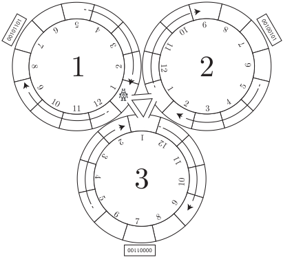
Loops. The Loops domain puts together all the previous examples. A robot can move on K loops of length L, in each loop there is a counter of B bits initialized at a random number. Fig. 1 shows an example with K = 3 loops of length L = 12 and with counters of B = 8 bits. Each cell in the loop is indexed from 1 to L. Each loop's counter is at cell ⌈L/2⌉ + 1. A robot can only move clockwise in the loop. When the robot is in cell 1 it can move in cell 1 of another loop. When in counter's cell, the robot can increase the counter by one. The goal is to have all the counters with the same value.

6.2 Analysis

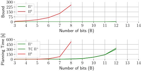
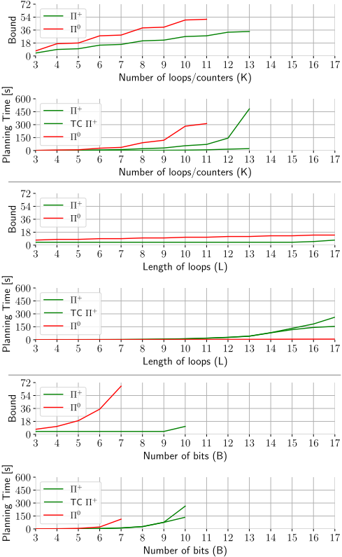
For each domain presented and for each problem of increasing size, we compare two encodings: Π+, i.e., the encoding presented in this paper employing the TC to execute (possibly) more than one action in one step, and Π0 , i.e., the approach presented in Thm. 3, where at most one action can be executed at each step. For both encodings, the PDDL domain and problem files (i.e., the planning task Π) are first encoded into Π+ and Π0 , and then translated into propositional formulae as shown in Eq. 1, starting from n = 0. We implemented the approach on the PATTY solver 3 [Cardellini et al., 2024] which makes use of Z3 v4.12.2 [de Moura and Bjørner, 2008] to compute the model (if any) satisfying Π+n and Π0n . Each problem and encoding has a time limit of 10 minutes on an Intel Xeon Platinum 8000 3.1GHz with 8GB of RAM. The results for the Counter, Cube and Loops domains are shown in Figs. 2, 3 and 4, respectively. For each domain, we show how the bound and planning time change while varying the size of the problem. The red line represents Π0 and the green line Π+. For the planning time, we consider the time elapsed from the parsing of the PDDL problem to the output of the plan. We indicate with a dashed green line the time it takes to compute the TC of all the actions in the planning task. The transitive closure is computed via BDDs, employing the pyeda tool 4 . In the BDD the variables in X ∪ X ′ have been ordered alphabetically by name. We limit the computation of all actions' TCs to 3 minutes, equally divided among all actions, and for each action we return the last computed transition relation before the time limit.

In the Counter domain, we recall that a valid plan must contain at least 2B - 1 incr actions. In Fig. 2 we see how, in fact, the bound required by Π0 to find a plan increases exponentially with B. For Π+ instead, the bound is 1 for B ∈ [3, 11] where the TC can be computed under the time limit. When B is 12 the TC computation reaches the time-limit and T 10 incr is returned, modelling 210 repetitions of incr (Lem. 1), and requiring a bound of 4 to find the valid plan of 212 - 1 repetitions. Notably, when the fix point is reached, the total time is mainly the time to compute the TC.

3 https://pattyplan.com

4 https://pyeda.readthedocs.io/

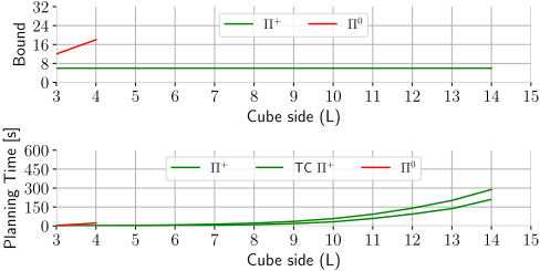
In the Cube domain, the shortest valid plan has 6×(L-1) actions which are reflected in the bound required by Π0 in Fig. 3. When L = 5 the bound required by Π0 would be 24, but the system timeouts before being able to find a solution. For Π+ instead, the TC can be computed under the time-limit until L = 15. Due to the amo+(A) axioms of the encoding, the bound for Π+ is equal to 6, i.e., the different actions in the plan. As discussed in Sec. 4.3, the use of constraints can allow, in some cases, the transitive closure to be smaller. Indeed, comparing the transitive closure size (in terms of BDD nodes) of the planning task with and without constraints, we obtain a 40% reduction in the BDDs nodes of the TC.

In the more complicated Loops domain, for each dimension, i.e., K, L and B, we plot how the bound and planning time change by varying one dimension and keeping the other one fixed to their minimum value (i.e., 3). By increasing the number of loops and counters (i.e., K), we see in the first and second chart from the top of Fig. 4, how the bounds for both Π+ and Π0 increase linearly with K. However, the bound of Π0 diverges linearly from the one of Π+, since, for each loop, a valid plan has L = 3 actions to move through the loop and at most 23 - 1 increases of the associated counter. By only increasing the length of the loops L in the third and fourth chart from the top, we see how again the bound of Π0 is greater than the bound of Π+. However, in this case, the planning time of Π0 is shorter than Π+, since, for smaller bounds, the computation of the TC is actually pricier than iteratively increasing the bound. The fifth and sixth charts present the same behaviour of the Counter domain.

In all the domains we have experimentally confirmed Thm. 6, showing that Π+ ≤ Π0 .

7 Conclusions and FutureWork

We presented a technique to perform rolling in classical planning with CEs and constraints, which was previously unexplored. We theoretically and experimentally demonstrated that the approach is interesting and beneficial. Several works have been published introducing new approaches to reduce the bound required to find a solution, being one of the weaknesses of the PaS approach [Wehrle and Rintanen, 2007; Balyo, 2013; Bofill et al., 2016; Cardellini et al., 2024; Cardellini and Giunchiglia, 2025]. In the future, we plan to (i) minimize the bound even further by integrating our TC approach in the latest SOTA PaS approach [Cardellini et al., 2024] where a finite sequence of actions is employed to apply different actions in the same step and (ii) study how to compute the TC of multiple actions, effectively combining the possible effects of different actions in one transition relation.

Acknowledgments

Matteo Cardellini and Enrico Giunchiglia were each partially supported by the projects FAIR (PE00000013) and SERICS (PE00000014), respectively, under the NRRP MUR program funded by the EU - NGEU.