
Participatory Budgeting Project Strength via Candidate Control
Proceedings of the Thirty-Fourth International Joint Conference on Artificial Intelligence. Main Track. Pages 3821-3829.
https://doi.org/10.24963/ijcai.2025/425
Keywords
- Game Theory and Economic Paradigms: GTEP: Computational social choice
Abstract
We study the complexity of candidate control in participatory budgeting elections. The goal of constructive candidate control is to ensure that a given candidate wins by either adding or deleting candidates from the election (in the destructive setting, the goal is to prevent a given candidate from winning). We show that such control problems are NP-hard to solve for many participatory budgeting voting rules, including Phragmén and Equal-Shares, but there are natural cases with polynomial-time algorithms. We also argue that control by deleting candidates is a useful tool for assessing the performance (or, strength) of initially losing projects, and we support this view with experiments on real-life PB instances.
- 1787 2098 645 1603 1467 1058 1459 1501 1957 1229 1018 1490 926 1560 1043 1644 640 1462 1949 1557 1573 1075 638 184 641 1806 1432 1619 639 2209 637 668 1554 1115 985 1551 1534 1072 1531 2257 Losing projects 210 264 300 1061 346 635 1034 349 1010 1027 1024 1556 344 643 1110 659 1967 1106 2209 1806 1619 1432 641 184 1075 1573 1557 1501 1957 1459 1490 1467 926 1644 1058 1043 1462 1603 2098 645 1949 1560 1229 1018 1787 640 638 639 637 668 985 1115 1534 2257 1551 1554 1072 1531 Rivals 0.0 0.2 0.4 0.6 0.8 1.0 Probability of winning (a) GREEDYAV 210 264 1644 1806 2098 1229 1459 1501 2209 1787 1432 1957 1462 Losing projects 1024 1061 300 346 635 1034 1560 1058 1573 1075 184 349 1010 926 1557 1027 637 1490 344 1556 1018 1043 1603 1467 639 641 643 645 659 1619 1110 1072 1551 1949 640 638 985 1115 1967 1534 1106 668 2257 1554 1531 1432 1806 2209 210 264 1501 1644 1787 2098 1229 1459 1957 1462 Rivals 0.0 0.2 0.4 0.6 0.8 1.0 Probability of winning (b) GREEDYCOST 1806 1644 1459 926 1787 1501 2098 1957 1229 1490 1018 1560 1058 1603 210 639 184 1462 1573 1467 Losing projects 264 2209 300 346 1432 635 1061 1024 1034 637 1075 349 1043 1557 1010 1619 645 641 1027 1949 640 638 1556 344 1072 1573 643 1110 1462 985 668 659 1551 210 1967 1115 1534 1106 1554 1531 1603 1806 1490 1957 1560 1058 1644 1501 1787 2098 1229 1018 926 1459 639 2257 184 1467 Rivals 0.0 0.2 0.4 0.6 0.8 1.0 Probability of winning (c) EQUAL-SHARES 210 264 1644 1806 2098 1787 1459 1501 1229 1957 2209 926 1490 1432 Losing projects 1024 1061 1058 300 346 1034 349 184 1075 635 1573 1560 1462 1010 1018 1557 1027 637 1556 344 1043 1467 1603 639 641 643 645 659 1619 1110 1551 1072 1949 640 638 985 1534 1967 1115 668 2257 1106 1554 1531 2209
- [Bartholdi III et al., 1992] John J. Bartholdi III, Craig A. Tovey, and Michael A. Trick. How hard is it to control an election? Mathematical and Computer Modelling, 16(8- 9):27-40, 1992.
- [Baumeister and Hogrebe, 2023] Dorothea Baumeister and Tobias Hogrebe. On the complexity of predicting election outcomes and estimating their robustness. SN Computer Science, 4(4):362, 2023.
- [Baumeister et al., 2021] Dorothea Baumeister, Linus Boes, and Johanna Hillebrand. Complexity of manipulative in- terference in participatory budgeting. In Proceedings of the 7th International Conference on Algorithmic Decision Theory, ADT '21, volume 13023 of LNCS, pages 424-439, 2021.
- [Boehmer et al., 2021] Niclas Boehmer, Robert Bredereck, Piotr Faliszewski, and Rolf Niedermeier. Winner robust- ness via swap-and shift-bribery: Parameterized counting complexity and experiments. In Proceedings of the 30th International Joint Conference on Artificial Intelligence, IJCAI '21, pages 52-58, 2021. IJCAI
- [Boehmer et al., 2023] Niclas Boehmer, Piotr Faliszewski, Łukasz Janeczko, and Andrzej Kaczmarczyk. Robustness of participatory budgeting outcomes: Complexity and ex- periments. In Proceedings of the 16th International Sym- posium on Algorithmic Game Theory, SAGT '23, volume 14238 of LNCS, pages 161-178, 2023.
- [Boehmer et al., 2024] Niclas Boehmer, Piotr Faliszewski, Łukasz Janeczko, Dominik Peters, Grzegorz Pierczyński, Šimon Schierreich, Piotr Skowron, and Stanisław Szufa. Evaluation of project performance in participatory budget- ing. In Proceedings of the 33rd International Joint Con- ference on Artificial Intelligence, IJCAI '24, pages 2678- 2686, 2024. IJCAI
- [Bredereck et al., 2021] Robert Bredereck, Piotr Fal- iszewski, Andrzej Kaczmarczyk, Rolf Niedermeier, Piotr Skowron, and Nimrod Talmon. Robustness among multiwinner voting rules. Artificial Intelligence, 290, 2021.
- [Brill et al., 2024] Markus Brill, Rupert Freeman, Svante Janson, and Martin Lackner. Phragmén's voting methods and justified representation. Mathematical Programming, 203(1):47-76, 2024.
- [Cabannes, 2004] Yves Cabannes. Participatory budgeting: A significant contribution to participatory democracy. En- vironment and Urbanization, 16(1):27-46, April 2004.
- [Erdélyi et al., 2015a] Gábor Erdélyi, Michael R. Fellows, Jörg Rothe, and Lena Schend. Control complexity in Bucklin and fallback voting: A theoretical analysis. Jour- nal of Computer and System Sciences, 81(4):632-660, 2015.
- [Erdélyi et al., 2015b] Gábor Erdélyi, Michael R. Fellows, Jörg Rothe, and Lena Schend. Control complexity in Bucklin and fallback voting: An experimental analysis. Journal of Computer and System Sciences, 81(4):661-670, 2015.
- [Faliszewski and Rothe, 2016] Piotr Faliszewski and Jörg Rothe. Control and bribery in voting. In Handbook of Computational Social Choice, pages 146-168. Cambridge University Press, 2016.
- [Faliszewski et al., 2009] Piotr Faliszewski, Edith Hemas- paandra, and Lane A. Hemaspaandra. How hard is bribery in elections? Journal of Artificial Intelligence Research, 35:485-532, 2009.
- [Faliszewski et al., 2023] Piotr Faliszewski, Jaroslaw Flis, Dominik Peters, Grzegorz Pierczyński, Piotr Skowron, Dariusz Stolicki, Stanisław Szufa, and Nimrod Talmon. Participatory budgeting: Data, tools and analysis. In Pro- ceedings of the 32nd International Joint Conference on Ar- tificial Intelligence, IJCAI '23, pages 2667-2674, 2023. IJCAI
- [Goel et al., 2019] Ashish Goel, Anilesh K. Krishnaswamy, Sukolsak Sakshuwong, and Tanja Aitamurto. Knapsack voting for participatory budgeting. ACM Transactions on Economics and Computation, 7(2):8:1-8:27, 2019.
- [Gonzalez, 1985] Teofilo F. Gonzalez. Clustering to mini- mize the maximum intercluster distance. Theoretical Com- puter Science, 38:293-306, 1985.
- [Hemaspaandra et al., 2007] Edith Hemaspaandra, Lane A. Hemaspaandra, and Jörg Rothe. Anyone but him: The complexity of precluding an alternative. Artificial Intelli- gence, 171(5-6):255-285, 2007.
- [Janeczko and Faliszewski, 2023] Łukasz Janeczko and Pi- otr Faliszewski. Ties in multiwinner approval voting. In Proceedings of the 32nd International Joint Conference on Artificial Intelligence, IJCAI '23, pages 2765-2773, 2023. IJCAI
- [Liu et al., 2009] Hong Liu, Haodi Feng, Daming Zhu, and Junfeng Luan. Parameterized computational complexity of control problems in voting systems. Theoretical Computer Science, 410(27-29):2746-2753, 2009.
- [Los et al., 2022] Maaike Los, Zoé Christoff, and Davide Grossi. Proportional budget allocations: Towards a sys- tematization. In Proceedings of the 31st International Joint Conference on Artificial Intelligence, IJCAI '22, pages 398-404, 2022. IJCAI
- [Magrino et al., 2011] Thomas R. Magrino, Ronald L. Rivest, Emily Shen, and David Wagner. Computing the margin of victory in IRV elections. Presented at 2011 Elec- tronic Voting Technology Workshop/Workshop on Trust- worthy Elections, August 2011.
- [Meir et al., 2008] Reshef Meir, Ariel D. Procaccia, Jef- frey S. Rosenschein, and Aviv Zohar. Complexity of strategic behavior in multi-winner elections. Journal of Artificial Intelligence Research, 33:149-178, 2008.
- [Peters and Skowron, 2020] Dominik Peters and Piotr Skowron. Proportionality and the limits of welfarism. In Proceedings of the 21st ACM Conference on Economics and Computation, EC '20, pages 793-794, 2020.
- [Peters et al., 2021] Dominik Peters, Grzegorz Pierczyński, and Piotr Skowron. Proportional participatory budgeting with additive utilities. In Proceedings of the 35th An- nual Conference on Neural Information Processing Sys- tems, NeurIPS '21, pages 12726-12737, 2021.
- [Rey and Maly, 2023] Simon Rey and Jan Maly. The (com- putational) social choice take on indivisible participatory budgeting. Technical Report arXiv.2303.00621, arXiv, 2023.
- [Shiryaev et al., 2013] Dmitry Shiryaev, Lan Yu, and Edith Elkind. On elections with robust winners. In Proceed- ings of the 12th International Conference on Autonomous Agents and Multiagent Systems, AAMAS '13, pages 415- 422, 2013.
- [Xia, 2012] Lirong Xia. Computing the margin of victory for various voting rules. In Proceedings of the 13th ACM Conference on Electronic Commerce, EC '12, pages 982- 999, 2012.
- [Yang, 2019] Yongjie Yang. Complexity of manipulating and controlling approval-based multiwinner voting. In Proceedings of the 28th International Joint Conference on Artificial Intelligence, IJCAI '19, pages 637-643, 2019. IJCAI
References were extracted automatically from the PDF and may contain errors.
Full text extracted automatically from the PDF; figures, tables and equations may differ. The PDF is the version of record.
1 Introduction
Participatory budgeting is a recent democratic innovation where cities allow their inhabitants to decide about a certain fraction of their budgets [Cabannes, 2004; Goel et al., 2019; Rey and Maly, 2023]. Specifically, some of the community members propose possible projects to be implemented and, then, all the citizens get a chance to vote as to which of them should be funded. Most commonly, such elections use approval ballots, where people indicate which projects they would like to see implemented, and the GREEDYAV rule, which selects the most approved projects (subject to not exceeding the budget). However, there also are more advanced rules, such as PHRAGM´EN [Brill et al., 2024; Los et al., 2022] or EQUAL-SHARES [Peters and Skowron, 2020; Peters et al., 2021], which produce arguably more fairor, to be precise, more proportional-decisions [Faliszewski et al., 2023]. Yet, with more advanced rules come issues about understanding the results. Indeed, recently Boehmer et al. [2024] have argued that proposers whose projects were rejected may find it quite difficult to understand the reasons for these outcomes. To alleviate this problem, they introduced a number of performance measures-mostly based on the bribery family of problems [Faliszewski et al., 2009; Faliszewski and Rothe, 2016]-that attempt to answer the following question: As a proposer of a project that was not funded, what could I have done differently to have it funded? For example, they ask if the project would have been funded if its cost were lower (see also the work of Baumeister et al. [2021]), or if its proposer convinced more people to vote for it, or if the proposer motivated some voters to only approve his or her project. Similar briberystyle problems were also used to evaluate the robustness of election results [Shiryaev et al., 2013; Bredereck et al., 2021; Boehmer et al., 2021; Baumeister and Hogrebe, 2023; Boehmer et al., 2023], or the margin of victory for the winners [Magrino et al., 2011; Xia, 2012].
In this paper, we follow-up on these ideas, but using candidate control. The main difference is that instead of focusing on circumstances that depend on a project's proposer (indeed, the project's cost is his or her choice, and it is his or her choice what support campaign he or she runs), we focus on external ones, independent of his or her actions (such as some other projects being submitted or not 1 ). We believe that looking at both types of reasons for a project's rejection gives a more complete view of its performance.
Candidate Control. The idea of the control-in-elections family of problems is that we are given a description of an election, a designated candidate, and we ask if it is possible to ensure that this candidate is a winner (in constructive control) or ceases to be a winner (in destructive control) by modifying the structure of the election [Bartholdi III et al., 1992; Faliszewski and Rothe, 2016]. Specifically, researchers consider control by adding or deleting either candidates or voters (some papers-including the one that introduced election control [Bartholdi III et al., 1992]-also consider various forms of arranging run-off elections as a type of control). So far, election control was mostly studied theoretically, with a focus on the complexity analysis [Bartholdi III et al., 1992; Hemaspaandra et al., 2007; Meir et al., 2008; Liu et al., 2009; Erd´elyi et al., 2015a; Yang, 2019], but some empirical results exist as well [Erd´elyi et al., 2015b]. We study candidate control in participatory budgeting, that is, we ask if it is possible to ensure funding of a given project (or, preclude its funding) by either adding new projects-from some a'priori known set of projects-or by deleting them. Our results are theoretical and focus on the complexity of our problems, but we motivate them by project performance analysis and we also show some experimental results that provide examples of such analysis. As our performance analysis is based on control by deleting projects, we pay most attention to results regarding this variant of control, and we include the addition case for the sake of completeness and to be in sync with the preceding literature.
1 We disregard the possibility that a proposer might try to discourage other people from proposing projects, albeit we acknowledge that this may happen, and this might even be quite benign: A group of activists focused on making their city more green may discuss among themselves which projects to submit and which to withhold.
| unit | unary | binary | ||||
|---|---|---|---|---|---|---|
| Del | Add | Del | Add | Del | Add | |
| GREEDYAV | P‡ | P‡ | P‡ | P‡ | NP-c | NP-c |
| GREEDYCOST | P‡ | P‡ | P‡ | P‡ | NP-c | NP-c |
| PHRAGM ´EN | NP-c | NP-c | NP-c | NP-c | NP-c | NP-c |
| EQUAL-SHARES | NP-c | NP-c | NP-c | NP-c | NP-c | NP-c |
Performance Analysis. Let us now discuss how one could use control by deleting candidates to analyze the performance of projects in participatory budgeting (we will use the terms projects and candidates interchangeably, e.g., using "candidates" in the names of control problems). Consider a participatory budgeting election and some not-funded project p. One basic measure of its performance is the smallest number of other projects that have to be removed from the election for p to be funded. The lower this number, the closer was the project to winning: Indeed, perhaps some proposers only managed to submit their projects in the last minute and it was possible that they would have missed the deadline, or some projects were close to being removed from the election due to formal reasons, but the city officials were not strict in this regard. However, it is more likely that such issues would affect cheaper projects than the more expensive ones-which, likely, had more careful proposers-so instead of asking for a smallest set of projects to delete, we may ask for a set with the lowest total cost.
Another way of using control by deleting projects to assess a project's performance is to use a probabilistic approach, along the lines of the one taken by Boehmer et al. [2021], Boehmer et al. [2023], and Baumeister and Hogrebe [2023] for bribery: We ask for the probability that project p is funded, assuming that a random subset of projects (of a given cardinality) is removed. The higher it is, and the lower the number of removed projects, the closer p is to winning.
A different interpretation of the above measures is that instead of thinking that some projects "barely made it" to participate in the election, we learn how many projects performed better than p. The more projects we need to delete to have p funded (or, to have p funded with sufficiently high probability) the more projects can be seen as critically stronger than p.
Finally, we can use candidate control as a way of assessing rivalry between projects. For example, if project p has a much higher probability of being funded after deleting a random set of projects under the condition that some other project q was included in this set, then we can view q as a strong rival of p.
Our Contributions. We provide theoretical and experimental results. First, we regard the complexity of candidate control for four well-known voting rules, depending on how the costs of the projects are encoded (either in binary, or in unary, or as unit costs, which means that each project costs the same amount). We show the overview of our results in Table 1. We mention that all our NP-hardness results also imply #P-hardness for respective problems where we ask for a number of solutions (e.g., number of ways in which we can ensure a victory of a given project by deleting a given number of others). This is interesting because solving such problems is necessary for estimating the probability that a project wins if a given randomly-selected set of projects is deleted. On the experimental side, we provide an analysis of real-world participatory budgeting instances, showing what one can learn about them via candidate control. To this end, we provide several performance measures and prove their usefulness in an extensive analysis of instances from PabuLib [Faliszewski et al., 2023]. The full version of the paper and the code for our experiments are available at https://github.com/ProjectPRAGMA/PB-control-IJCAI-2025.
2 Preliminaries
An instance of participatory budgeting (PB) is a triple E = (P, V, B), where P = {p1, . . . , pm} is a set of projects, V = {v1, . . . , vn} is a set of voters, and B ∈ N is an available budget. Each voter v ∈ V is associated with an approval set A(v) ⊆ P , which is the set of projects they approve. For each project p ∈ P, we know cost(p) ∈ N, cost(p) ≤ B, i.e., the price for which this project can be implemented. We extend this notation from a single project p to a set of projects S ⊆ P and set cost(S) = ∑p∈S cost(p). We say that S ⊆ P is a set of B-feasible projects if cost(S) ≤ B.
A PB rule is a function f : E → 2P that, for a given PB instance, outputs a B-feasible subset of projects. Note that we assume the rules to be resolute, which can be easily ensured by incorporating some tie-breaking order into them. Let W = f(E) for some rule f and some PB instance E. We say that projects from W are selected or, equivalently, funded. The projects not in W are called losing.
In this work, we consider four different participatory budgeting rules. Each of these rules starts with an empty set W and sequentially, in rounds, extends W with additional projects unless the budget B is exhausted or all the projects were processed. More formally, given a PB instance E = (P, V,B), the rules of our interest works as follows:
GREEDYAV. We define the score of a project p ∈ P as the number of voters approving p; formally scoreAV(p) = |{v ∈ V | p ∈ A(v)}|. The GREEDYAV rule then processes the projects in non-increasing order according to their scores (with ties resolved according to a given tiebreaking order). If the rule can afford the currently processed project p, i.e., cost(W) + cost(p) ≤ B, then it includes p in W. Otherwise, the rule continues with the next project. The rule terminates when all projects were processed.
GREEDYCOST. This rule is very similar to the GREEDYAV rule. The only difference is in the order in which the projects are processed. Specifically, the score of a project p ∈ P under GREEDYCOST rule is scoreAV/C(p) = scoreAV(p)/ cost(p). The process is then identical as in the GREEDYAV rule.
PHRAGM´EN. This rule is conceptually different from the two above. Here, each voter starts with an empty virtual bank account, which is, in a continuous manner, increased by one unit of money per unit of time. Once there is a project p ∈ P \ W such that the sum of balances of voters approving p is exactly cost(p), the current round ends, and the rule performs several steps. First, it includes project p into the set of funded projects. Next, it sets the balance of all voters approving p to zero. Finally, the rule removes all projects p′ ∈ P \ W such that cost(W) + cost(p′ ) > B. Then, the rule continues with the next round. The rule terminates when there is no remaining project in P .
EQUAL-SHARES. Our last rule is also based on the idea of virtual bank accounts. However, this time, the budget is proportionally spread between the voters, meaning that each voter starts with the initial balance of B/n, and this initial value is never increased. Again, the rule works in rounds. In each round, the rule funds a project such that its supporters have enough cumulative budget to fund this project, and each of them covers as small a fraction of its cost as possible. Formally, let bi be the current balance of a voter vi. We say that a project p ∈ P \W is q-affordable, where q ∈ [0, 1], if
In each round, the rule funds a project that is q-affordable for the smallest q over all projects and adjusts the balances of voters supporting p: Specifically, the balance bi of each agent is decreased by qi · cost(p), where qi = q if bi > q · cost(p) and bi/ cost(p) otherwise. The rule terminates when no affordable project exists.
It is known that the EQUAL-SHARES rule is not exhaustive [Peters et al., 2021]. In our experiments, we use the Add1 completion: If the EQUAL-SHARES outcome is not exhaustive, we increase each voter's budget by 1 and rerun the rule. We do so until we get an exhaustive outcome or find an outcome that exceeds the original budget (and take the nonexhaustive solution from the previous iteration in this case).
Control Problems. We focus on the control by adding or deleting projects and follow the standard notation from single- and multi-winner voting [Faliszewski and Rothe, 2016]. Let f be a PB rule. In the f-CONSTRUCTIVE CONTROL BY DELETING CANDIDATES (f-CCDC, for short), we are given an instance E = (P, V,B) of PB, an integer r, and a project p ̸∈ f(E), and our goal is to decide whether it is possible to delete a set D of at most r such that p ∈ f((P \ D, V,B)). In the f-DESTRUCTIVE CONTROL BY DELETING CANDIDATES (f -DCDC), the project p is initially funded, and the goal is to decide whether we can delete at most r projects so that project p becomes a loser.
In control by adding projects, there are two disjoint sets of projects: P is a set of standard projects, and Q is a set of spoiler projects. The rule does not initially consider the spoiler projects. The question here is whether we can find at most r spoiler projects such that once we add them to the instance, then project p is (in the case of f-CCAC) or is not (in the case of f -DCAC) funded by the rule f.
In our algorithmic results, we are sometimes interested in the weighted variant of the above-defined problems. Under this consideration, each project p is additionally associated with its weight ω(p), and the goal is to decide whether a set D of projects securing our goal exists such that ∑p∈D ω(p) ≤ r. We indicate the weighted variant by adding a dollar sign in front of the operation type. For example, the weighted variant of f -CCDC is referred to as f -CC$DC. Even though the weighted variant might seem unnatural at first glance, the motivation for it is two-fold. First, it is studied in the literature on control in elections [Faliszewski and Rothe, 2016]. Second, and more importantly, if we set the weight of each project equal to its cost, we can use a hypothetical algorithm for the weighted variant to find a set of the lowest total costs that secures our goal, one of the proposed performance measures.
3 Complexity Results
Due to space restrictions, we focus on the complexity picture of both constructive and destructive control by deleting projects. This operation is arguably more natural for reallife instances and is also assumed in our experimental results. Before we present our results, let us illustrate the concept of control by deleting projects using a toy example.
Example 1. Assume an instance with three projects c1, c2, and p. Project c1 is approved by three voters, project c2 by two voters, and project p by a single voter. The costs of the projects are cost(c1) = 1, cost(c2) = 2, and cost(p) = 1. The total budget is B = 2. Under the GREEDYAV rule, project c1 is considered first, and since its cost is smaller than the budget, this project gets funded. Next, the rule considers project c2, but this project costs more than the remaining budget. Lastly, project p is considered and eventually also funded. If we remove project c1, then project c2 gets funded and exhausts the budget, and therefore, project p cannot be funded. Hence, removing c1 from the instance is a successful destructive control that prevents p from winning and a successful constructive control that makes c2 winning.
We start with the GREEDYAV rule. In our first result, we show that both constructive and destructive control are computationally intractable, even if the instance is unweighted. Maybe surprisingly, this hardness result holds even if the instance contains only two agents. We give a reduction from the classic NP-complete [Gonzalez, 1985] problem RX3C, in which we are given a universe U = {u1, . . . , u3N} and a family S of 3N size-3 subsets S1, . . . , S3N ⊂ U such that every element ui ∈ U appears in exactly 3 subsets of S, and we ask if there are N subsets in S whose union is U.
Theorem 1. Both GREEDYAV-CCDC and GREEDYAVDCDC are NP-complete, even if |V | = 2.
Proof Sketch. The idea of the proof is that the projects are in 1-to-1 correspondence with the sets, and using project costs, we encode which elements are covered by each set. We achieve this by having project costs as a 3N digit-length number in base 4. A project pj corresponding to a subset Sj = {ui1 , ui2 , ui3 } ∈ S, i1 < i2 < i3, then has cost of the form
where the i-th digit of this cost has value one if and only if the element ui belongs to Sj. All other digits are always zero. Next, we set the budget and the cost of our distinguished project p so that it gets funded only if the deleted projects correspond to subsets that form an exact cover in I.
Formally, given an instance I = (U, S), we construct an instance J of GREEDYAV-CCDC as follows. For each set Sj ∈ S, Sj = {ui1 , ui2 , ui3 }, we create a set-project pj with cost 1 · 4i1 + 1 · 4i2 + 1 · 4i3 . Next, we add our distinguished project p and N + 1 guard-projects g1, . . . , gN+1. The cost of the distinguished project p is ∑3N i=1 1 · 4i and for every i ∈ [N+1], we set cost(gi) = cost(p)+1. That is, the guard projects are only one unit more expensive compared to our distinguished project. This ensures that the budget left after we delete some set-projects is exactly the cost of p.
The set of voters consists of just two voters, v1 and v2. The first voter, v1, approves all projects except for p. The second voter, v2, approves only the set-projects. Such a preference profile secures that, regardless of the tie-breaking order, the method first processes all set-projects, then all guard-projects, and only as the last possibility, the method processes the distinguished project p.
To complete the construction, we set B = ∑3N i=1 3 · 4i and r = N. Observe that the number of guard-projects is one greater than the number of projects we are allowed to delete; hence, no solution may delete all guard-projects. The budget is selected so that if we do not delete any project, all the setprojects are funded, and the budget is exhausted after the last set-project is taken into consideration by the rule. On the other hand, if we remove N projects corresponding to subsets forming an exact cover in I, the remaining budget after the rule processes all the set-projects will be exactly the cost of p.
First, let us show that p is indeed initially not funded. The scoreAV of every set-project pj, j ∈ [3N], is exactly two, the scoreAV of the guard-projects is exactly one, while the scoreAV of our distinguished project p is zero. Therefore, all other projects are processed before project p. Moreover, their total cost is ∑3N i=1 3 · 4i due to the definition of the costs and the fact that every element ui appears in exactly three subsets. Therefore, when the distinguished project p is processed by the rule, the budget is B-∑3N i=1 3·4i = ∑3N i=1 3·4i -∑3N i=1 3· 4i = 0. Hence, project p is clearly not affordable.
For left-to-right implication, let I be a YES-instance and let C ⊂ S be an exact cover of U. We delete every setproject pj such that Sj ∈ C, and we claim that p is now founded, that is, the control is successful. Since C is an exact cover, we spend exactly ∑3N i=1 2 · 4i on the set-projects. Consequently, after the last set-project is processed by the rule, the remaining budget is B- ∑3N i=1 2·4i = ∑3N i=1 3 · 4i - ∑3N i=1 2·4i = ∑3N i=1 (3-2)·4i = ∑3N i=1 1·4i . This is one unit of money less than the cost of any guard-project. Therefore, no guard-project is funded, and once the rule processes p, the remaining budget is still ∑3N i=1 1 · 4i which is the cost of p, so p is funded. Consequently, J is also a YES-instance.
The hardness construction from Theorem 1 requires prices of exponential size. That is, our problems are, from the computational complexity perspective, weakly NP-hard. It is natural to ask whether Theorem 1 can be strengthened to polynomial-size prices or if a pseudopolynomial time algorithm exists for the problem. In the following result, we answer this question positively by giving an algorithm based on dynamic programming, which works even in the case of weighted control.
Theorem 2. If the costs of the projects are encoded in unary, both GREEDYAV-CC$DC and GREEDYAV-DC$DC can be solved in polynomial time, even if the projects' weights are encoded in binary.
Proof Sketch. Our algorithm is based on the dynamic programming approach. We present an algorithm for constructive control; for destructive control, only a minor tweak is required when we are checking the table for the existence of a solution.
We suppose that p1, . . . , pm-1, p is the order in which the rule processes the projects in the original instance; that is, p1 is processed first and pℓ is processed just before the distinguished project p. Note that the assumption that p is processed last is not in contradiction with the fact that our algorithm works for any tie-breaking order, as we can remove all projects that the GREEDYAV rule processes after the distinguished project p. Moreover, we can remove all projects with cost(pj) > B, as such projects cannot be afforded.
The central part of the algorithm is to compute a dynamic programming table DP[j, β], where j ∈ [m-1] is an index of the last processed project, and β ∈ [B] is a desired remaining budget just before the rule processes a project pj+1. We call the pair (j, β) a signature. For every signature, the dynamic programming table stores the weight of a minimum-weight partial solution Dj,β ⊆ {p1, . . . , pj} such that if the projects fromDj,β are removed, the remaining budget just before the GREEDYAV rule processed project pj+1 is exactly β. If no such partial solution exists, we store some large value ∞ (in fact, it is enough to store a value greater than r).
The computation is then defined as follows. The basic step is when j = 1. Here, we just decide whether p1 needs to be deleted or not, based on the required remaining budget β. Formally, we set the dynamic programming table as follows:
For every j ∈ [2,m-1], the computation of the algorithm is defined as follows.
The first case corresponds to a situation where we need to decide whether to include pj in a solution or not. In the second case, we cannot fund pj anyway, so we need not delete it, and we are only interested in whether the same budget can be achieved just before pj is processed. In the last case, we cannot delete pj , as it would exceed the budget.
Once all the cells of the dynamic programming table DP are correctly computed, we can decide the instances. Specifically, we return YES whenever there exists a cell DP[m1, β], where β ≥ cost(p), such that DP[m- 1, β] ≤ r. The dynamic programming table has O(m · B) cells, and each cell can be computed in time O(log(r)). The final check can be done in O(B) time; therefore, the overall running time of the algorithm is O((m · B) · log(r) +B), which, assuming the unary-encoded budget, is clearly a polynomial-time algorithm, even if the projects' weights are encoded in binary.
Theorem 2 implies that for real-life elections, performance measures based on project control can be computed efficiently.
The hardness construction provided in Theorem 1 and the algorithm from Theorem 2 also work for the GREEDYCOST rule. For the former result, one can observe that even under the GREEDYCOST rule, the property that the set-projects are processed before the guard-projects, and that the guardprojects are processed before the distinguished project p is preserved. This comes from the fact that set-projects are approved by exactly two voters, guard-projects by exactly one voter, and p by no voter. Moreover, no set-project is more expensive than any guard-project. The algorithms require that the relative ordering of the projects is not affected by deletions. This is also clearly preserved under GREEDYCOST.
Corollary 1. Both GREEDYCOST-CCDC and GREEDYCOST-DCDC are NP-complete, even if |V | = 2. If the projects' costs are encoded in unary, even the weighted control can be solved in polynomial time.
Now, we turn our attention to the PHRAGM´EN rule. Here, the situation is significantly less positive. Specifically, in the following theorem, we show that for this rule, it is NP-hard to decide whether successful control is possible, even if the instance is unweighted and all projects are of the same cost.
Theorem 3. Both PHRAGM´EN-CCDC and PHRAGM´ENDCDC are NP-complete, even if the projects are of unit cost.
The idea behind the construction is that we have one project for every set Si ∈ S in RX3C instance and many direct competitors of the distinguished project p. The setprojects have significantly higher support than p or its competitors, and, moreover, the competitors of p share their voters with the set-projects. Hence, all the set-projects are always funded before the first project of a different type may be funded. These set-projects exhaust most of the budget, and unless every voter approving a competitor of p approves a funded set-project, the remainder of the budget is spent on the competitor of p, which is, consequently, not funded.
To finalize the complexity picture, we show that for the EQUAL-SHARES rule, the control by deleting projects is also highly intractable. To prove this result, we exploit a reduction of Janeczko and Faliszewski [2023], who showed that it is NP-hard to decide whether the EQUAL-SHARES rule outputs the same outcome for every tie-breaking order.
Theorem 4. Both EQUAL-SHARES-CCDC and EQUALSHARES-DCDC are NP-complete, even if the projects are of unit cost.
For performance measures based on the probability that a project wins/loses if a randomly selected set of projects is deleted or added, it is essential to efficiently determine the number of solutions for an instance. However, it turns out that all our NP-hardness results, excluding EQUAL-SHARES and the deletion operation, also imply #P-hardness for respective problems. Therefore, we do not expect the existence of a significantly faster algorithm for computing such measures than a simple enumeration of all possible solutions.
4 Experiments
We analyze the effect of project deletions on real-world data from Pabulib [Faliszewski et al., 2023] and explore how different performance measures based on this operation can help with understanding and explanation of outcomes for proposers of losing projects and PB election organizers.
Data. In our experiments, we analyze 543 approval-based PB instances from Pabulib. We include every instance with approval ballots available as of October 2024 with at least one losing project. In total, our dataset contains 10531 losing projects for GREEDYAV, 5771 for GREEDYCOST, 6004 for PHRAGM´EN, and 7412 for EQUAL-SHARES. The largest instance consists of 160 projects and 90494 voters.
Experimental Setup. The experiments were run on computers with two AMD EPYC™ 7H12, 64-core, 2.6 GHz CPUs, and 256 GB DDR4 3200MT/s RAM. We use the same Python implementation for rules GREEDYAV, GREEDYCOST, and PHRAGM´EN as in [Boehmer et al., 2024]. For EQUAL-SHARES, we use our own implementation in C++ that significantly outperforms the available implementations. For each rule, every instance, and every combination of r ∈ {1, 2, 3} projects in this instance, we determined the winners after deleting these r projects. Evaluating the instances with our rules took us the following number of core-hours: 38000 for PHRAGM´EN, 900 for both GREEDYAV and GREEDYCOST, and 5000 for our C++ implementation of EQUALSHARES. The overall running time is significantly skewed by instances with many projects, as we need to try all O(nr ) subsets (recall that significant speed-up for these rules is not possible due to Theorems 3 and 4). For computing the optimal control in the setting with either GREEDYAV or GREEDYCOST, we use the DP algorithm from Theorem 2, which finishes for the whole dataset in less than 1 core-hour.
4.1 HowClose is a Project to Being Funded?
In general, PB rules do not provide any information about the performance of proposed projects-a project is either funded or not-and there are no direct ways of measuring how close a project was to being successful. Indeed, this is exactly what drove Boehmer et al. [2024] to initiate the study of project performance measures. Here, we propose several further measures based on constructive control by deleting projects.
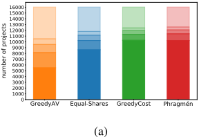
The first, very basic, approach we suggest is to count how many other projects need to be removed from the instance to make some initially losing project p funded. In Figure 1a, we present an overview of the results for the whole dataset. For GREEDYAV, more than 47% initially losing projects get funded after the removal of at most 3 projects; for the remaining rules, the value is smaller, but still significant - 37%
for GREEDYCOST, 40% for EQUAL-SHARES, and 43% for PHRAGM´EN, respectively. Another interesting information we gain from Figure 1a is that for most of the projects for which it is enough to remove at most three projects, it is actually enough to remove only one other project. This is most evident in the case of GREEDYAV.
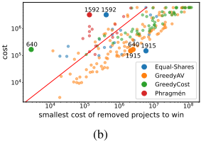
Yet, saying that a project is close to winning simply because it can be funded after deleting some small number of carefully selected projects is overly simplistic. On the one hand, it is not too surprising that a project gets selected after deleting some other, expensive projects. On the other hand, we expect such expensive projects to be well-prepared and not to be removed for formal reasons, or due to missing a deadline. Consequently, instead of taking the number of projects that we need to delete to get some initially losing project p funded, we may rather seek the cheapest set of projects (of a given cardinality) whose deletion gets p funded. This measure indeed is much more fine-grained than our first one. To see this, we consider the results for Warsaw, Citywide, 2023 PB election, shown in Figure 1b: There are certain projects where the removal of expensive projects is the only way to get them funded (e.g., project 1915), but there are also projects that get funded after removing rather cheap projects (see, e.g., project 1592). Note that this behavior is not very consistent among different PB rules, which is caused mostly by their underlying principles: whether the rule is more proportionality- or social-welfare-oriented (e.g., to get project 640 funded, we delete cheaper projects under GREEDYCOST, but more expensive ones under GREEDYAV).
Both above measures have the downside that they focus on deleting exactly a particular subset of projects. However, even if we can get some initially losing project p to be funded after deleting projects whose cost is X, it is possible that p would be losing after deleting some other projects, whose cost is 2X (while this may seem unintuitive, it can happen due to various possible interactions among the projects and involved operation of our PB rules). Hence, in the remainder of this section, we take a more stochastic approach and analyze the probability that a project gets funded if we remove a random subset of projects of some predefined size. We start with an overview of the whole dataset, and later we analyze one specific instance to show what information can be gained from measures based on the probability of winning.
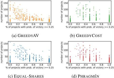
In Figure 2, we have a data point for every instance and plot the percentage of initially losing projects that have at least 25% probability of being funded after the removal of three random projects. First, we see that for all the voting rules, there are instances where successful control is either unlikely for large fractions of projects or, on the contrary, where control is likely to be successful for nearly all projects. This affects more frequently instances of smaller size. Also, there is a visible difference between GREEDYAV and the remaining rules: unlike in GREEDYAV, for these rules, the instances are more 'clustered' around certain percentage values, while for GREEDYAV, the instances are more spread.
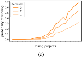
Now, we focus on a specific instance. In Figure 1c, we plot for each losing project of the instance Warsaw, Ursynow, 2019 (under GREEDYAV), the probability that this project becomes a winner if r projects are removed for different values of r. From this plot, we can distinguish between projects that are 'clear losers', meaning that their probability of winning is very close to zero regardless of the size of the removal set, and projects that are much closer to winning. This demonstrates how useful such a measure of a project's strength is.
4.2 Who Are My Biggest Rivals?
The performance measures introduced so far allow us to compare projects from a 'global perspective', meaning that we can see how a losing project performed relative to other losing projects. However, for project proposers, it is very important to know why their project was not funded and what can be done to improve their project's performance in the future. One possibility is to identify a given project's rivals-projects whose removal significantly increases its chances of victory. Proposers of losing projects can then analyze such rivals, learn what they did differently, and improve their projects.
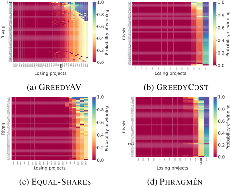
We propose the following measure of rivalry. We set the r-rivalry between a losing project p and some other project q equal to the probability that p is funded after we remove q and r other random projects. In Figure 3, we present the results for r = 2, instance Warsaw, Ursynow, 2019, and different PB rules. It is not surprising that the strongest rivals are usually the projects that were initially funded. However, this is not always the case. One such example is project 1490 under the PHRAGM´EN rule (Figure 3d), for which the (initially losing) project 1432 is a much stronger rival than most of the initially winning projects. It can also be the case that for some projects, their funding relies solely on the performance of a few other projects. A very good example of this behavior is project 1806 under the GREEDYAV rule (Figure 3a): unless we remove project 210, there is almost no chance that project 1806 will ever be funded. This measure also nicely complements the measures from the previous subsection, as, based on plots similar to Figure 3, we can visually distinguish projects that are hopeless losers, which are somewhere in the middle, and which projects almost got in.
5 Conclusions
In our experiments, we demonstrated the usefulness of project performance analysis. One can use our measures to compare different projects and provide election organizers with information on which projects were very close to being funded. In practice, cities often try to discuss popular losing projects and fund them from an increased or completely separate budget. Moreover, our rivalry measures help project proposers identify which other projects prevented their success. If such strong rivals share some similarities, the proposer can learn from them and improve their project for the next round of PB.
Our work's most immediate extensions are to study approximation and parameterized algorithms for the corresponding hard computational problems and to extend our experiments also to winning projects.
Ethical Statement
Even though our paper's goal is to improve the explainability and transparency of participatory budgeting outcomes, voting control is traditionally understood as malicious and highly undesired behavior. As such, one might object that our work could increase awareness of possible manipulation in PB elections. We want to stress that manipulations based on our performance measures are implausible: Our measures can be computed only after the elections have ended and we have complete (and anonymized) information about the whole instance. That is, the potential knowledge based on our measures can be used, if at all, to manipulate the next installation of PB elections. However, the new instance will most likely be different since some projects have already been funded, new projects will be proposed, and, in particular, voters' preferences may change over time.
Acknowledgments
We would like to thank the anonymous reviewers for their helpful comments. This project has received funding from the European Research Council (ERC) under the European Union's Horizon 2020 research and innovation programme (grant agreement No 101002854). Łukasz Janeczko's research presented in this paper is supported in part from the funds assigned by Polish Ministry of Science and Technology to AGH University. This work was co-funded by the European Union under the project Robotics and advanced industrial production (reg. no. CZ.02.01.01/00/22 008/0004590). This work was supported by the Ministry of Education, Youth and Sports of the Czech Republic through the eINFRA CZ (ID: 90254), project OPEN-30-16. Jan Pokorn´y and ˇSimon Schierreich acknowledge the additional support of the Grant Agency of the CTU in Prague, grant No. SGS23/205/OHK3/3T/18.


@inproceedings{ijcai2025p425,
  title     = {Participatory Budgeting Project Strength via Candidate Control},
  author    = {Faliszewski, Piotr and Janeczko, Łukasz and Knop, Dušan and Pokorný, Jan and Schierreich, Šimon and Słuszniak, Mateusz and Sornat, Krzysztof},
  booktitle = {Proceedings of the Thirty-Fourth International Joint Conference on
               Artificial Intelligence, {IJCAI-25}},
  publisher = {International Joint Conferences on Artificial Intelligence Organization},
  editor    = {James Kwok},
  pages     = {3821--3829},
  year      = {2025},
  month     = {8},
  note      = {Main Track},
  doi       = {10.24963/ijcai.2025/425},
  url       = {https://doi.org/10.24963/ijcai.2025/425},
}
TY - CPAPER TI - Participatory Budgeting Project Strength via Candidate Control AU - Faliszewski, Piotr AU - Janeczko, Łukasz AU - Knop, Dušan AU - Pokorný, Jan AU - Schierreich, Šimon AU - Słuszniak, Mateusz AU - Sornat, Krzysztof T2 - Proceedings of the Thirty-Fourth International Joint Conference on Artificial Intelligence, IJCAI-25 PB - International Joint Conferences on Artificial Intelligence Organization PY - 2025 SP - 3821 EP - 3829 DO - 10.24963/ijcai.2025/425 UR - https://doi.org/10.24963/ijcai.2025/425 ER -Copied
Machine-readable versions of this paper, for tools and AI agents:





