
Towards the 30 by 30 Kunming-Montreal Global Biodiversity Framework Target: Optimising Graph Connectivity in Constraint-Based Spatial Planning
Proceedings of the Thirty-Fourth International Joint Conference on Artificial Intelligence. AI and Social Good. Pages 9772-9780.
https://doi.org/10.24963/ijcai.2025/1086
Keywords
- Multidisciplinary Topics and Applications: General
- Constraint Satisfaction and Optimization: General
- Planning and Scheduling: General
Abstract
The Kunming-Montreal Global Biodiversity Framework aims to protect 30% of terrestrial, inland water, marine, and coastal ecosystems worldwide, and ensuring that at least 30% of these areas are under effective restoration by 2030.
Maintaining and restoring ecological connectivity between natural habitats and protected areas is a key feature of this target.
Achieving it will require effective and inclusive spatial planning supported by appropriate decision-support tools.
Most spatial planning models address budget as an objective and connectivity as a constraint, formulating problems with Steiner trees.
In many real-world cases, such as landscape-scale restoration planning, this formulation is inappropriate when environmental managers seek to optimise connectivity under a budget constraint.
This problem was previously addressed with Constraint Programming (CP) and graph variables, but the current approach is severely limited in terms of spatial resolution.
In this article, we formalise this problem as the budget-constrained graph connectivity optimisation problem. Based on a real case study: the restoration of forest connectivity in New Caledonia, we illustrate why ``naive'' CP approaches are inefficient.
In response, we provide a preprocessing method based on Hanan grids which preserves the existence of at least one optimal solution.
Finally, we assess the efficiency of our approach in the New Caledonian case study.
- [Alagador et al., 2012] Diogo Alagador, Maria Triviño, Jorge Orestes Cerdeira, Raul Brás, Mar Cabeza, and Miguel Bastos Araújo. Linking like with like: Optimis- ing connectivity between environmentally-similar habi- tats. Landscape Ecology, 27(2):291-301, February 2012.
- [Bessière et al., 2015] Christian Bessière, Emmanuel Hébrard, George KATSIRELOS, and Toby Walsh. Reasoning about Connectivity Constraints. In IJCAI: International Joint Conference on Artificial Intelligence, pages 2568-2574. AAAI Press, July 2015. IJCAI
- [Birnbaum et al., 2015] Philippe Birnbaum, Thomas Ibanez, Robin Pouteau, Hervé Vandrot, Vanessa Hequet, Elodie Blanchard, and Tanguy Jaffré. Environmental correlates for tree occurrences, species distribution and richness on a high-elevation tropical island. AoB PLANTS, 7, January 2015.
- [Birnbaum et al., 2024] Philippe Birnbaum, Jeremy Girardi, Dimitri Justeau-Allaire, Thomas Ibanez, Vanessa Hequet, Nathan Eltabet, and Juliette Prior. Forest Map of New Caledonia, July 2024.
- [CBD, 2022] CBD. Kunming-Montreal Global Biodiversity Framework (CBD/COP/15/L.25). Convention on Biologi- cal Diversity. 2022. 2022.
- [Conrad et al., 2012] Jon M. Conrad, Carla P. Gomes, Willem-Jan van Hoeve, Ashish Sabharwal, and Jordan F. Suter. Wildlife corridors as a connected subgraph prob- lem. Journal of Environmental Economics and Manage- ment, 63(1):1-18, January 2012.
- [Daigle et al., 2020] Rémi M. Daigle, Anna Metaxas, Arieanna C. Balbar, Jennifer McGowan, Eric A. Treml, Caitlin D. Kuempel, Hugh P. Possingham, and Maria Beger. Operationalizing ecological connectivity in spatial conservation planning with Marxan Connect. Methods in Ecology and Evolution, 11(4):570-579, 2020.
- [Dilkina et al., 2017] Bistra Dilkina, Rachel Houtman, Carla P. Gomes, Claire A. Montgomery, Kevin S. McK- elvey, Katherine Kendall, Tabitha A. Graves, Richard Bernstein, and Michael K. Schwartz. Trade-offs and efficiencies in optimal budget-constrained multispecies corridor networks. Conservation Biology, 31(1):192-202, February 2017.
- [Dooms et al., 2005] Gregoire Dooms, Yves Deville, and Pierre Dupont. CP(Graph): Introducing a Graph Compu- tation Domain in Constraint Programming. In Principles and Practice of Constraint Programming -CP 2005, Lec- ture Notes in Computer Science, pages 211-225. Springer, Berlin, Heidelberg, October 2005.
- [Fages, 2015] Jean-Guillaume Fages. On the use of graphs within constraint-programming. Constraints, 20(4):498- 499, October 2015.
- [Ganley and Cohoon, 1994] Joseph L Ganley and James P Cohoon. Routing a multi-terminal critical net: Steiner tree construction in the presence of obstacles. In Pro- ceedings of IEEE International Symposium on Circuits and Systems-ISCAS'94, volume 1, pages 113-116. IEEE, 1994.
- [Garey and Johnson, 1977] M. R. Garey and D. S. John- son. The rectilinear steiner tree problem is $np$-complete. SIAM Journal on Applied Mathematics, 32(4):826-834, 1977.
- [Hanan, 1966] Maurice Hanan. On steiner's problem with rectilinear distance. SIAM Journal on Applied mathemat- ics, 14(2):255-265, 1966.
- [Huang and Young, 2013] Tao Huang and Evangeline FY Young. Obsteiner: An exact algorithm for the construc- tion of rectilinear steiner minimum trees in the presence of complex rectilinear obstacles. IEEE Transactions on Computer-Aided Design of Integrated Circuits and Sys- tems, 32(6):882-893, 2013.
- [Jafari et al., 2017] Nahid Jafari, Bryan L. Nuse, Clinton T. Moore, Bistra Dilkina, and Jeffrey Hepinstall-Cymerman. Achieving full connectivity of sites in the multiperiod re- serve network design problem. Computers & Operations Research, 81:119-127, May 2017.
- [Jaffré et al., 1994] T Jaffré, P Morat, and JM Veillon. La flore de nouvelle-calédonie. Caractéristiques et composi- tion floristique des principales formations végétales. Bois et Forêts des Tropiques, 242:8-28, 1994.
- [Justeau-Allaire and Prud'homme, 2022] Dimitri Justeau- Allaire and Charles Prud'homme. Global domain views for expressive and cross-domain constraint programming. Constraints, January 2022.
- [Justeau-Allaire et al., 2021] Dimitri Justeau-Allaire, Ghis- lain Vieilledent, Nicolas Rinck, Philippe Vismara, Xavier Lorca, and Philippe Birnbaum. Constrained optimization of landscape indices in conservation planning to support ecological restoration in New Caledonia. Journal of Ap- plied Ecology, 58(4):744-754, 2021.
- [Justeau-Allaire et al., 2023] Dimitri Justeau-Allaire, Jef- frey O. Hanson, Guillaume Lannuzel, Philippe Vismara, Xavier Lorca, and Philippe Birnbaum. Restoptr: An R package for ecological restoration planning. Restoration Ecology, page e13910, 2023.
- [Justeau-Allaire et al., 2025] Dimitri Justeau-Allaire, Sulian Le Bozec-Chiffoleau, Xavier Lorca, Charles Prud'homme, gilles simonin, Philippe Vismara, Philippe Birnbaum, Nicolas Rinck, and nicolas beldiceanu. dimitri- justeau/optgraphcon: Data and source code for "towards the 30 by 30 kunming-montreal global biodiversity frame- work target: Optimising graph connectivity in constraint- based spatial planning", May 2025.
- [Justeau-Allaire, 2023] Dimitri Justeau-Allaire. AI and Spa- tial Planning for Sustainable Socio-Ecosystems. In Thirty- Second International Joint Conference on Artificial Intel- ligence {IJCAI-23}, page 6370. International Joint Con- ferences on Artificial Intelligence Organization, August 2023.
- [Lehtomäki and Moilanen, 2013] Joona Lehtomäki and Atte Moilanen. Methods and workflow for spatial conservation prioritization using Zonation. Environmental Modelling & Software, 47:128-137, September 2013.
- [McGarigal and Marks, 1995] Kevin McGarigal and Bar- bara J. Marks. FRAGSTATS: Spatial pattern analysis pro- gram for quantifying landscape structure. Gen. Tech. Rep. PNW-GTR-351. Portland, OR: U.S. Department of Agri- culture, Forest Service, Pacific Northwest Research Sta- tion. 122 p, 351, 1995.
- [Prud'homme and Fages, 2022] Charles Prud'homme and Jean-Guillaume Fages. Choco-solver: A Java library for constraint programming. Journal of Open Source Soft- ware, 7(78):4708, October 2022.
- [Rehfeldt and Koch, 2023] Daniel Rehfeldt and Thorsten Koch. Implications, conflicts, and reductions for steiner trees. Mathematical Programming, 197(2):903-966, 2023.
- [Zachariasen, 2001] Martin Zachariasen. A catalog of hanan grid problems. Networks: An International Journal, 38(2):76-83, 2001.
References were extracted automatically from the PDF and may contain errors.
Full text extracted automatically from the PDF; figures, tables and equations may differ. The PDF is the version of record.
1 Introduction
The world faces an unprecedented biodiversity crisis due to human activities, with land use changes being the most damaging. While only two Sustainable Development Goals (SDGs) explicitly address biodiversity (SDG 14: life below water, SDG 15: life on land), most relate indirectly to ecosystem health [Justeau-Allaire, 2023]. In this regard, the recent Kunming-Montreal Global Biodiversity Framework (GBF) aims to stop biodiversity loss and promote sustainable societies. Two of its targets, also known as "30 by 30", aim to ensure that, by 2030, (i) at least 30% of areas of degraded terrestrial, freshwater, marine, and coastal ecosystems are under effective restoration, and (ii) at least 30% of terrestrial, freshwater, marine, and coastal ecosystems are conserved and managed [CBD, 2022]. The Kunming-Montreal GBF also acknowledges that inclusive and effective spatial planning is essential to achieve these goals, including cultural, social, economic, political, and ecological factors, with a focus on maintaining and restoring ecological connectivity.
Over the past few decades, many spatial planning models have been devised and applied to incorporate connectivity into biodiversity conservation and restoration projects. Such models usually rely on heuristics [Lehtomäki and Moilanen, 2013], metaheuristics [Daigle et al., 2020], Mixed-Integer Linear Programming (MILP) [Jafari et al., 2017], or Constraint Programming (CP) [Bessière et al., 2015]. Declarative approaches such as MILP or CP are particularly relevant in spatial planning because they allow the design of flexible and expressive decision-support tools that can adapt to different situations and support iterative co-construction processes with stakeholders. Indeed, such approaches are built upon generic and exact problem-solving mechanisms, which makes it possible to enrich and modify a decision-support model without affecting the solving procedure or losing satisfiability and optimality guarantees.
In most spatial planning models, ecological connectivity is treated as a constraint, and a budget representing either an economic cost or a biodiversity metric is optimised. This problem is equivalent to the Steiner Tree problem and has been addressed as such in several studies [Conrad et al., 2012; Alagador et al., 2012; Bessière et al., 2015; Dilkina et al., 2017]. These contributions are important and have greatly advanced our capacity to support better conservation and restoration strategies. However, after a decade of close collaboration with environmental managers in New Caledonia for forest conservation and restoration projects, we can state that this formulation is often not appropriate. In fact, environmental managers usually have limited budgets and need to account for many constraints related to land accessibility and opportunity costs. They have to plan conservation and ecological restoration programs at landscape scales, where it is rarely possible to satisfy strict connectivity constraints given these limited budgets. In such cases, minimising costs often leads to recommendations that have hardly any chance of leading to concrete action, since, even if the cost is minimal, it cannot be supported by the community. A counterargument can be made in favour of promoting long-term conservation and restoration plans, but the functioning of public funding and their strong dependence on electoral calendars rarely guarantee the continuation of a plan over the long term. In such situations, it is therefore preferable to guarantee the feasibility of a conservation or restoration project, while optimising its ecological benefits.
This article introduces the Budget-Constrained Connectivity Optimisation (BCCO) problem, which is highly relevant to spatial planning. The goal is to optimise the connectivity of an ecological network (e.g., natural habitats, protected areas) while adhering to a budget limit. It has been tackled in several CP-based spatial planning models [JusteauAllaire et al., 2021; Justeau-Allaire et al., 2023], but never formalised. The flexibility and expressiveness of CP, notably through the graph variable paradigm [Dooms et al., 2005; Fages, 2015], are indeed naturally adapted to express this problem and its variants, but efficient solving remains tedious with a "naive" CP approach. In related work, a degradation of the spatial resolution of the input data was always necessary, leading to a loss of information and less accurate decision support. Indeed, the BCCO problem is NP-Hard and therefore needs to be formalised and equipped with theoretical and practical results to enable scaling up.
In the following, we first formalise the BCCO problem and prove its NP-Hardness. We then present related work, referred to as naive CP models, and illustrate their lack of efficiency in a real case study: reforestation of mining sites in New Caledonia. To overcome these limitations, we introduce a preprocessing method based on Hanan grids that preserves the existence of an optimal solution. This preprocessing step allows us to address larger instances of the problem without degrading their spatial resolution. We finally illustrate this result in the New Caledonian case study and discuss the perspectives it offers for biodiversity conservation and ecological restoration planning.
2 The Budget-Constrained Connectivity Optimisation (BCCO) Problem
In spatial planning problems, we represent a geographic area of interest by a set of planning units (PUs) constituting a tessellation of this area. Most often, the PUs correspond to a regular square grid, but they can also correspond to other types of regular grids, e.g. hexagonal, or to irregular grids, e.g. cadastral parcels. We can naturally define an adjacency relationship as the geometric adjacency between PUs. Given that, we can represent the area of interest by an undirected graph G = (V, E), where V corresponds to the set of PUs and E to the set of adjacent pairs of PUs. In ecological restoration and protected areas network extension problems, a set T ⊆ V is given as input and depicts existing habitat areas (respectively protected areas). By analogy with the Steiner tree problem, nodes in T are named the terminals. An integer cost is associated with each node x, denoted by cV (x). Finally, using the P(G) notation to depict the power set of G, we define the connectivity metric connect : P(G) ↦→ N as the number of connected components of a subgraph of G. This metric corresponds to the number of patches (NP) metric in Landscape Ecology [McGarigal and Marks, 1995]. It is noteworthy that because edges reflect a geometric adjacency relationship, for any subgraph G′ = (V ′ ,E′ ) ⊆ G, the set E′ is directly induced by V ′ (there is necessarily an edge between any two spatially adjacent nodes). We can therefore use the notation of induced subgraphs: G′ = G[V ′ ]. Given this, we formally define the BCCO problem.
Definition 1 (The BCCO problem). Let G = (V,E) be a graph, T ⊆ V a subset of nodes (the terminals), cV : V ↦→N be a cost function over the nodes of G, and B be a maximum budget. The BCCO problem expresses as follows:
Proposition 1. The BCCO problem is NP-Hard.
Proof. Let BCCD be the decision version of BCCO whose instances are made of a graph G, a subset of nodes T, a cost function cV over the nodes and two integers C and B. The question is: Is there a subgraph of G, containing T, such that the number of connected components is less than C and whose total cost is less than B? We consider the NodeWeighted Steiner Tree (NWST) problem, known to be NPComplete, whose instances are made of a graph GS , a subset of nodes T S , a cost function cSV over the nodes and an integer K. The question is: Is there a connected subgraph of GS , containing T S , such that the total cost is less than K? One can notice that NWST is a particular case of BCCD (C = 1). Thus, the polynomial transformation is trivial. This proves that BCCD is NP-Hard. Since BCCO is obviously NPO, we obtain that BCCO is NP-Hard.
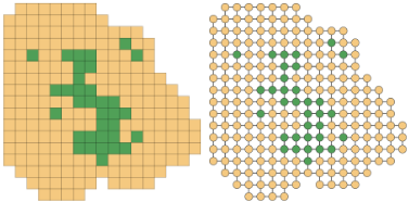
In our case, we will consider geographic areas tessellated with a regular square grid (from raster data, Figure 1a), equipped with the four-connected adjacency relationship. Also, we set the same unit cost to all PUs, so cV (x) = 1 ∀x ∈ V . This leads to a partial grid graph representation of the geometric area (Figure 1b). The NP-Hardness result still holds for that case, as we can reduce the Rectilinear Steiner Tree (RST) problem, which is NP-Complete [Garey and Johnson, 1977], to BCCD.
(a) Raster representation. (b) Graph representation.
Figure 1: Raster and graph representation of a geographic area using the four-connected adjacency relation; terminals are in green.
3 Illustration of the Naive CP Approach in a New Caledonian Case Study
The previous CP approaches to the BCCO problem can be described as "naive" in the sense that they do not take advantage of the relationships between the budget, the connectivity metric, and the geometric properties of the problem. The main limitation of such approaches is that they are only effective in instances with poor spatial resolution. To illustrate this, we rely on the case study introduced in [JusteauAllaire et al., 2023], which consists in planning reforestation actions in the Kaala Mount mining area in New Caledonia. Like most New Caledonian mining areas, the Kaala Mount is home to a high diversity of plant species. Indeed, more than 3200 native vascular plant species can be found in New Caledonia, most being endemic (≈75%) [Jaffré et al., 1994; Birnbaum et al., 2015]. However, in such mining areas, this biodiversity is under severe threat, and therefore, mining companies have a legal obligation to invest in ecological restoration in their operating zones.
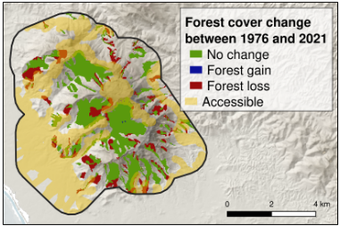
In the Kaala Mount case study, the aim was to restore the forest fragmentation level of 1976, based on an expert forest digitisation from 1976 aerial images and an automated 2021 forest digitisation from Landsat satellite images time series. Since the publication of the Kaala Mount case study, an updated map of New Caledonian forests was published [Birnbaum et al., 2024]. This map was digitised by experts from aerial images that have a much higher spatial resolution than Landsat satellite images. Therefore, it is better adapted for comparison with the 1976 forest map, notably because the automated approach can confuse shrubland with forest. The comparison between the 1976 forest and this updated 2021 forest map shows a net forest area loss of ≈354 ha (see Figure 2). We rely on this updated dataset, which we rasterised to a spatial resolution of 30m × 30m (0.09 ha), to formulate a BCCO problem instance:
With a maximum budget corresponding to 20% of the forest cover loss that occurred between 1976 and 2021 in the Kaala Mount mining area (≈ 71 ha), identify accessible areas to reforest in order to minimize forest fragmentation. Accessible areas are defined by a 150 m buffer around existing tracks, and the forest fragmentation is measured as the number of forest patches.
By following the graph transformation method illustrated in Figure 1 and by aggregating all connected terminals into one single terminal node, we construct the graph GS = (T ∪ A, E) with T the set of forest patches in the 2021 map, corresponding to the terminals, and A the set of pixels located in accessible areas not covered by forest. Given that, the base naive BCCO CP model, as defined in [Justeau-Allaire et al., 2021; Justeau-Allaire et al., 2023], is composed of a nodeinduced graph variable GH = (VH,EH) ∈ [GS[T],GS], the habitat graph, and a node-induced subgraph view GR = GH[VH \ T], the restoration graph (see [Justeau-Allaire and Prud'homme, 2022] for more details on subgraph views). Then, a budget integer variable b ∈ [0,B] is defined such that b = ∑x∈R c(x), with c the cost function corresponding to PUs' restorable areas and the set variable R being a view on the nodes of GR. Finally, we define an integer variable NCC = connect(GH) ∈ [1, |T|], which is the number of connected components (number of patches) of the habitat graph, and set as the optimisation objective to minimise. Thanks to the expressiveness of CP and its ability to handle abstract and complex mathematical constructs, this model is highly compact and readable.
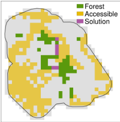
We implemented this model using Choco-solver [Prud'homme and Fages, 2022] and ran it on an Ubuntu laptop (Intel Core i7-12700H × 20; 32GB of RAM), setting a time limit of 10h. As expected, the solver could not complete the problem within the time limit. We therefore reduced the 30m × 30m spatial resolution of the input data using restoptr's aggregation method [Justeau-Allaire et al., 2023]. We repeated this procedure until the solver could solve the problem. This led us to an extremely degraded instance with pixels of 300m × 300m (see Figure 7a).
4 A PreprocessingMethod Based on Hanan Grids and Graph Reductions
The BCCO problem is similar to Steiner tree problems. Because we consider the restricted case of the regular square grid tessellation with unit costs, it resembles the Rectilinear Steiner Tree (RST) problem in the plane. More specifically, it resembles the Obstacle Avoiding Rectilinear Steiner Tree (OARST) problem [Ganley and Cohoon, 1994] as some PUs are not accessible and thus cannot be reforested.
In this section, we consider a version of the BCCO problem expressed in the plane instead of in the raster, we call it Rectilinear BCCO (R-BCCO). We present techniques for reducing the search space for R-BCCO inspired by what exists for OARST, and we exploit these techniques in the raster representation.
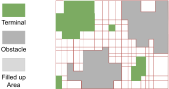
An instance I of R-BCCO is a plane containing complex rectilinear polygons that are either terminals or obstacles (Figure 3-left). These polygons are delimited by horizontal and vertical segments, called boundary edges. The boundary of a polygon is the set of points that belong to at least one of its boundary edges. The interior of a polygon is the set of points that belong to the polygon but not to its boundary.
The feasible region is the minimal rectangular region of the plane that contains all polygons. A feasible solution τ is a rectilinear forest , i.e. a union of disjoint rectilinear trees made up of horizontal and vertical segments that do not intersect with the interior of any polygon and that belong to the feasible region. The set of feasible solutions is denoted F(I). The total length of τ is denoted L(τ) and corresponds to the sum of the lengths of the segments that make it up. The length of a segment is the rectilinear distance between its two extremities. The set of terminals is denoted T . We define the function C : F(I) ↦→P (T), withP (T) the set of all partitions of T, where C(τ) is the set of maximal and disjoint subsets of terminals that are interconnected by segments of τ, either directly or via other terminals and segments of τ . These subsets are referred to as the connected components of τ. The connectivity connect : F(I) ↦→ N is the number of connected components of a feasible solution: connect(τ) = |C(τ)|.
Definition 2 (The R-BCCO problem). Let I be a plane with complex rectilinear terminals and obstacles. Given a maximum budget B ∈ N, R-BCCO is defined as follows:
Note that OARST consists in minimising L(τ) under the constraint that connect(τ) = 1. Theorems 1 and 2 stated in this section also hold for OARST.
4.1 The Complex Rectilinear Grid
The Hanan Grid [Hanan, 1966] plays an important role in solving the RST problem in the plane by transforming it into a graph problem of finite size. The idea is to draw vertical and horizontal lines from the terminals, which are points of the plane. This defines a region of the plane that contains at least one optimal solution to the optimisation version of RST. Then, a weighted graph is constructed from the grid. The nodes are the terminals and the intersection points between the lines, called Steiner points. An edge exists between two nodes if they lie on the same segment of the grid, and if no other node lies between them on that segment. The weight is the rectilinear distance between the two nodes. Many studies have been devoted to Hanan grids and graph transformations for variants of OARST. For example, [Ganley and Cohoon, 1994] introduced the concept of the Escape Graph when rectilinear obstacles are present; [Zachariasen, 2001] proposed a more general problem than RST, encompassing many variants of it, for which they showed that an optimal solution belongs to the Hanan grid; [Huang and Young, 2013] presented a more reduced graph, called the Virtual Graph, when obstacles are complex rectilinear polygons, not just rectangles.
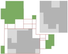
However, none of these works provide a reduced size grid when both terminals and obstacles are complex rectilinear polygons. We therefore propose a grid similar to the escape graph for this particular type of instance. Let I be a plane with complex rectilinear terminals and obstacles. The Complex Rectilinear grid CR(I) is obtained by taking all obstacle boundaries and constructing vertical and horizontal lines from each convex corner of terminals and obstacles. A convex corner of a rectilinear polygon is a corner in which the interior of the polygon forms a 90◦ angle. Inversely, a concave corner is a corner in which the interior of the polygon forms a 270◦ angle. Lines are extended until they hit a terminal or obstacle. Lines do not go along terminal boundaries. More formally, for any convex corner c, there is a unique horizontal (resp. vertical) segment h(c) (resp. v(c)), external to the polygon of c, that connects c to the boundary edge of a polygon (terminal or obstacle) or to an edge of the feasible region. Let CR(I) = BO ∪ ⋃c∈convex corners {h(c), v(c)}, with BO the set of obstacle boundary edges. See Figure 3-left.
Theorem 1. Let I be a plane with complex rectilinear terminals and obstacles, and B be a non-negative integer. CR(I) does contain an optimal solution to the R-BCCO problem.
Proof. The proof is inspired by [Ganley and Cohoon, 1994]. The idea is to consider an optimal solution and move it to CR(I) without making it unfeasible or non-optimal. Obviously, there is an optimal solution to R-BCCO within the feasible region. Let T ⊆ F(I) be the set of optimal solutions (i.e. minimising connect) of minimum total length, and let τ be a solution with minimum number of maximal segments among T . A maximal segment of τ is a segment that cannot be extended in τ. By definition, C(τ) = {C1, ...,Cconnect(τ)} is the set of subsets of T connected by τ, and let τ1, ..., τconnect(τ) be the trees of τ such that τk connects the terminals in Ck, with 1 ≤ k ≤ connect(τ).
Let s be a maximal segment of τ such that s does not belong to CR(I). Without loss of generality, say that s is horizontal. Let a be the number of vertical segments of τ above s that cross it, and b be the number of vertical segments of τ below s that cross it. τ is of minimum total length, so s cannot overlap a terminal boundary edge, as all points on the boundary of a same terminal are already connected. Thus, there is room to move s up or down.
If a > b (resp. a < b), then sliding s up (resp. down) by an infinitesimal distance, as well as the extremity of each vertical segment crossing s, would strictly decrease L(τ) while maintaining connect(τ) and the feasibility of τ. This contradicts the fact that τ has minimum total length, so a = b.
The edges of the feasible region belong to CR(I), so there is at least one horizontal line from CR(I) which is above s. Then, we slide s up until it encounters a line from CR(I), as well as the extremity of the vertical segments crossing s. Suppose that s hits a terminal boundary edge before a line from CR(I). In that case, s would overlap with a terminal boundary edge, and the overlapping part of s could be removed without disconnecting any terminal. This contradicts the fact that s is an optimal solution of minimum total length. Suppose that s hits another horizontal segment s′ of τ before a line from CR(I). Then, merging s with s′ would lead to an optimal solution that is either shorter in total length (if s ∩ s′ is a segment) or of the same length but with fewer maximal segments (if s∩s′ is a point). This contradicts the hypotheses about τ . Thus, s will necessarily hit a line from CR(I) first.
Because a = b and because no other horizontal segment of τ is crossed when sliding s up until it hits a line from CR(I), the total length of τ does not increase. If s does not touch any terminal, then moving s does not disconnect any terminals from Ck since the extremity of each vertical segment of τ crossing s is also moved. If an extremity of s touches a vertical boundary edge e of a terminal in Ck, the up-extremity of e is either a convex corner generating a line from CR(I) or a concave corner whose horizontal boundary edge is above s. Thus, s cannot be slid beyond the up-extremity of e, as it will hit a line from CR(I) before it happens. This proves that moving s to CR(I) does not disconnect any terminal in Ck and thus does not increase connect(τ), maintaining the optimality of τ .
The complex rectilinear grid in the raster representation.
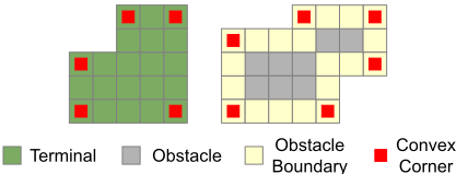
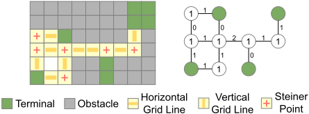
In practice, we will directly draw the complex rectilinear grid within the raster representation. By analogy with R-BCCO, a terminal is a block of terminal PUs connected in the fourconnected adjacency relationship, while an obstacle is a block of non-accessible PUs connected in the eight-connected adjacency relationship (where two diagonal pixels are connected). Terminal boundaries belong to terminals, so do the convex corners. While obstacle boundaries do not belong to obstacles, so the convex corners are on the outside of obstacles (see Figure 4). Lines are drawn from the convex corners, and drawing a line from a given pixel consists in scanning accessible pixels in one direction and marking them as a horizontal or vertical line of the grid. A Steiner point is a pixel marked as both a horizontal and a vertical grid line (see Figure 6). Theorem 1 also holds for the raster representation; the reasoning behind the proof is the same.
4.2 Reducing the Complexity of Obstacles
A key point in efficiently solving problems that rely on Hanan grids is to generate the fewest possible lines, as they represent the search space and thus the combinatorics of the problem. That is why we proposed the complex rectilinear grid CR(I)
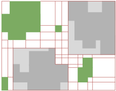
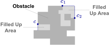
based on the particularities of our instances. However, we can further reduce the size of the resulting grid by transforming the instance itself. Indeed, lines are drawn from the convex corners of terminals and obstacles. Thus, finding an equivalent instance with fewer convex corners will reduce the size of the generated grid. With this in mind, we provide two rules to reduce the number of convex corners of the obstacles by filling them up (see Figure 5 for an illustration):
- 1) Let O be an obstacle, and c be one of its convex corners. Let us draw a line Lc from c. If Lc hits O without intersecting with any other obstacle, then let A be the area defined by Lc and the boundary of O. If no terminal nor other obstacle intersects with the interior of A, then merge it into O, filling it up.
- 2) Let O be an obstacle and (c1, c2) be two of its convex corners. Let us draw orthogonal lines Lc1 and Lc2 from c1 and c2. If these lines cross each other without intersecting with any other obstacle, then let A be the area defined by Lc1 , Lc2 and the boundary of O. If no terminal nor other obstacle intersects with the interior of A, then merge it into O, filling it up.
Apply these two rules until no area can be filled up, we call this procedure the filling procedure.
Theorem 2. The filling procedure converges in polynomial time and preserves the optimal value for R-BCCO.
Proof. Let B ∈ N and S be an optimal solution to R-BCCO. Let O be an obstacle and A be an area that can be filled up by rule 1) or 2). If S intersects with A, then let S′ be the solution obtained from S by moving S ∩ A to the boundary of O ∪A (O after filling up A). This does not disconnect any terminal nor increases the total length of S; thus S′ is also an optimal solution to R-BCCO. Also, every time rule 1) or 2) is applied, the number of convex corners decreases by at least one, so the procedure converges in polynomial time.
Remarks. The result of the filling procedure is not unique and depends on the order in which we consider the convex corners to which we apply rule 1) or 2). Theorem 2 also holds for the raster representation; the reasoning behind the proof is the same.
See Figure 3-middle for an illustration of the impact of the filling procedure on the search space.
4.3 Equivalent Graph
The idea of using Hanan grids is to transform the original instance in the plane into an instance in the graph. This way the search space becomes finite and a solution can be computed. The equivalent graph is composed of two types of nodes: a) a terminal node represents a complex rectilinear terminal, and b) a Steiner node represents a Steiner point, i.e. an intersection point between two lines of the grid. There is an edge in the graph when two nodes touch the extremities of the same grid segment, with no other node between them on the segment. The weight of the edge is the segment length. Multiple edges linking the same two nodes may appear because of the polygonal terminals, keep only the one of minimum weight.
The equivalent graph for the raster representation. In the raster, the grid lines have a non-zero width; thus we need to add weight to the nodes too. Terminal nodes have weight 0 while Steiner nodes have weight 1, and the length of a segment is the number of PUs separating its two extremities, as illustrated in Figure 6.
Once the graph is constructed, we can solve the BCCO problem. However, the graph now has weights on both nodes and edges, which is not the case in the original formulation. For this reason, we introduce the Weighted BCCO (W-BCCO) problem, a generalisation of BCCO. The connectivity function (connect) is the same as for BCCO.
Definition 3 (The W-BCCO problem). Let G be a simple and undirected graph. Let ωV : V (G) ↦→N and ωE : E(G) ↦→N
be weight functions on both nodes V (G) and edges E(G). Given a set of terminals T ⊆ V (G) and a maximum budget B ∈ N, W-BCCO expresses as follows:
We can construct an optimal solution S∗ to R-BCCO (resp. BCCO) in polynomial time from an optimal solution S∗W to W-BCCO in the equivalent graph. Each node in the graph corresponds either to a terminal or a Steiner point in the original instance.
- If a node v belongs to SW, then add the corresponding Steiner point or terminal to S∗ ;
- If an edge (u, v) belongs to S∗W , then add to S∗ a shortest path between u and v in the original instance.
It is easy to verify that S∗ is indeed an optimal solution to R-BCCO (resp. BCCO).
4.4 Reducing the Graph Size
After our instance has been transformed into a graph thanks to the complex rectilinear grid, the next preprocessing stage consists in reducing the graph size. Although graph reduction techniques for the Minimum Steiner Tree problem in the Graph (MSTG) have already been studied in the literature [Rehfeldt and Koch, 2023], we use three simple reduction rules for W-BCCO that exploit the fact that we do not need to retain all optimal solutions, but only at least one of them. Remember that both nodes and edges have a weight; we define the weight ω(P) of a path P from u to v as the sum of the weight of its edges and nodes, except the weights of u and v.
- Node removal: Let s be a Steiner node of degree at most one, remove it from the graph.
- Edge merging: Let s be a Steiner node of degree 2 with u and v its two neighbours. Create the edge (u, v) of weight ωE(u, v) = ωE(s, u) + ωE(s, v) + ωV (s), then remove s from the graph. If the edge (u, v) already exists, then keep only the one of minimum weight.
- Edge removal: Let (u, v) be an edge of the graph. If there is a path P from u to v of weight ω(P ) ≤ ωE(u, v) such that (u, v) /∈ P , then remove (u, v) from the graph.
Apply these three rules until no changes are made to the graph; we call this procedure graph simplification.
Theorem 3. Graph simplification converges in polynomial time and preserves the optimal value for W-BCCO.
Proof. It is rather straightforward to prove that each rule preserves the optimal value. Also, the size of the graph decreases by at least one whenever a change occurs after applying a rule, so the procedure converges in polynomial time.
Remark. Graph simplification does not alter the construction of an optimal solution in the original instance.
See Figure 3-right for an illustration of the impact of graph simplification on the search space.
5 Experiments on the Use Case
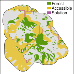
We implemented the preprocessing method described in Section 4 and applied it to the reforestation planning problem described in Section 3. We obtained an undirected graph with 1026 nodes and 1785 edges. Relying on this graph, we proposed the following CP model for the W-BCCO problem: Let G = (V,E) ∈ [G,G] be an undirected graph variable such that G is the set of terminal nodes, without edges, and G the graph obtained after the preprocessing method. We associate a set of Boolean variables BS with the Steiner nodes of G such that BS(x) = 1 if and only if x ∈ V . We also associate a set of Boolean variables BE with the edges of G, such that BE(x, y) = 1 if and only if (x, y) ∈ E. We define the budget with an integer variable b ∈ [0,B], with B the maximum budget, and such that b = ∑x∈V BS(x) + ∑(x,y)∈E BE(x, y) × ωE(x, y). Finally, the NCC ∈ [1, |T|] integer variable is defined such that NCC = connect(G) (number of patches), and set as the objective to minimise. We implemented this model using Choco-solver and ran it on a laptop (Intel Core i7-12700H × 20; 32GB RAM), setting the same 10h time limit as in Section 3. The preprocessing took ≈33s to complete, and the solver could find an optimal solution within no more than ≈1.6s. We finally projected this solution on the original raster grid by running a breadth-first search to associate a shortest path in the raster grid with each edge of the optimal solution to W-BCCO (see Figure 7b). The associated data and source code is available in Zenodo [Justeau-Allaire et al., 2025].
We show the impact of each step of the preprocessing procedure in Table 1 with the number of nodes and edges of the equivalent graph, the preprocess and solving times, and the value of the best solution found within 10h in three configurations: CR(I) only (CR); the filling procedure and then CR(I) (FP+CR); the filling procedure, CR(I) and then graph simplification (FP+CR+GS). The solving time is the time to find the best solution in CR and FP+CR (optimality was not reached), and to find and prove the optimal solution in FP+CR+GS. The graph for the naive CP model had 24 581 nodes.
(b) With preprocessing.
| CR | FP+CR | FP+CR+GS | |
|---|---|---|---|
| #Nodes | 18 082 | 3 044 | 1 026 |
| #Edges | 34 743 | 5 630 | 1 785 |
| Preprocess time | 0.09s | 1.14s | 32.68s |
| Solving time | 781.2s | 253.6s | 1.6s |
| #Patches (connect) | 81 | 72 | 65* |
Table 1: Statistics for the three configurations (* = optimal)
6 Discussion
In this study, designed by computer scientists, natural scientists, and environmental managers, we formalised the BCCO problem. This problem addresses concrete needs for biodiversity conservation and restoration planning. To overcome the current limitations of CP approaches to the BCCO problem, we proposed a polynomial time preprocessing method based on Hanan grids that greatly reduces the combinatorial complexity of our instances while preserving the existence of an optimal solution. We experimented with this approach on a real reforestation case study in New Caledonia and demonstrated the ability of this novel approach to tackle real instances without degrading the spatial resolution. This advance also opens up new challenges to fully take advantage of spatial planning problems properties. For instance, can we devise a filtering scheme taking advantage of the relationships between the budget variable and the connectivity metric which could be directly incorporated into the CP solving procedure? How can we express additional constraints (e.g. geometrical) on the graph obtained after the preprocessing procedure to allow for more expressiveness in problem formulation? Can we extend our approach to other metrics than connect? Etc. Nonetheless, this result is highly promising and provides many perspectives to provide better decision support in biodiversity conservation and restoration projects, especially given the current Kunming-Montreal 30 by 30 target. In particular, discussions with natural scientists and environmental managers suggest that our approach could also be used well ahead restoration actions and directly in the impact avoidance and reduction phases of mining projects.
Collaborations with stakeholders and domain experts. Codesigned by AI researchers, multi-disciplinary domain experts, and an environmental manager, this work is part of the [Justeau-Allaire, 2023] research project. This work builds on nearly 15 years of collaboration between the AMAP lab and forest conservation and restoration stakeholders in New Caledonia (e.g. Provinces, nonprofit organizations, mining companies). This long-term anchorage in the New Caledonian institutional landscape allows a fluid dialogue and mutual understanding of biodiversity and spatial planning challenges. The results presented in this article enable us to maintain this dialogue and to conduct concrete reflections on conservation and restoration policies while reducing the gap between management and science. Finally, this "living laboratory" configuration enables the production of tools and practices that are useful in other projects and in other parts of the world. For example, we are initiating similar approaches for restoring the Mesoamerican corridor in Panama and preserving and restoring tropical forests in Madagascar and Guinea.
Acknowledgments
This publication has emanated from research conducted with the financial support of the Futur & Ruptures program co-granted by IMT, Institut Carnot TSN, Institut Carnot M.I.N.E.S. and Fondation Mines-Télécom.
Contribution Statement
All the authors conceived the ideas and methodologies. Sulian Le Bozec-Chiffoleau (SLBC) and Dimitri Justeau-Allaire (DJA) led the writing of the manuscript. DJA, Philippe Birnbaum (PB), and Nicolas Rinck (NR) prepared the dataset and designed the case study. SLBC, DJA, Xavier Lorca (XL), Charles Prud'homme (CP), Gilles Simonin (GS), Philippe Vismara (PV), and Nicolas Beldiceanu (NB) designed the models and algorithms. DJA and SLBC implemented the models and algorithms, conducted the experiment and analysed its results. NR, PB, and DJA discussed the results and identified the perspectives for management. All the authors contributed critically to the draft and gave final approval for publication.
@inproceedings{ijcai2025p1086,
  title     = {Towards the 30 by 30 Kunming-Montreal Global Biodiversity Framework Target: Optimising Graph Connectivity in Constraint-Based Spatial Planning},
  author    = {Le Bozec-Chiffoleau, Sulian and Justeau-Allaire, Dimitri and Lorca, Xavier and Prud'homme, Charles and Simonin, Gilles and Vismara, Philippe and Birnbaum, Philippe and Rinck, Nicolas and Beldiceanu, Nicolas},
  booktitle = {Proceedings of the Thirty-Fourth International Joint Conference on
               Artificial Intelligence, {IJCAI-25}},
  publisher = {International Joint Conferences on Artificial Intelligence Organization},
  editor    = {James Kwok},
  pages     = {9772--9780},
  year      = {2025},
  month     = {8},
  note      = {AI and Social Good},
  doi       = {10.24963/ijcai.2025/1086},
  url       = {https://doi.org/10.24963/ijcai.2025/1086},
}
TY - CPAPER TI - Towards the 30 by 30 Kunming-Montreal Global Biodiversity Framework Target: Optimising Graph Connectivity in Constraint-Based Spatial Planning AU - Le Bozec-Chiffoleau, Sulian AU - Justeau-Allaire, Dimitri AU - Lorca, Xavier AU - Prud'homme, Charles AU - Simonin, Gilles AU - Vismara, Philippe AU - Birnbaum, Philippe AU - Rinck, Nicolas AU - Beldiceanu, Nicolas T2 - Proceedings of the Thirty-Fourth International Joint Conference on Artificial Intelligence, IJCAI-25 PB - International Joint Conferences on Artificial Intelligence Organization PY - 2025 SP - 9772 EP - 9780 DO - 10.24963/ijcai.2025/1086 UR - https://doi.org/10.24963/ijcai.2025/1086 ER -Copied
Machine-readable versions of this paper, for tools and AI agents:





