
Dual Contrastive Graph-Level Clustering with Multiple Cluster Perspectives Alignment
Proceedings of the Thirty-Third International Joint Conference on Artificial Intelligence. Main Track. Pages 3770-3779.
https://doi.org/10.24963/ijcai.2024/417
Keywords
- Machine Learning: ML: Clustering
- Machine Learning: ML: Unsupervised learning
Abstract
Graph-level clustering, which is essential in medical, biomedical, and social network data analysis, aims to group a set of graphs into various clusters. However, existing methods generally rely on a single clustering criterion, e.g., $k$-means, which limits their abilities to fully exploit the complex Euclidean and structural information inherent in graphs. To bridge this gap, we propose a dual contrastive graph-level clustering (DCGLC) method in this paper. DCGLC leverages graph contrastive learning and introduces the Euclidian-based and subspace-based cluster heads to capture the cluster information from different cluster perspectives. To overcome the inconsistency estimations and fuse the cluster information of multiple cluster heads, we propose a contrastive mechanism to align the cluster information derived from them. The cluster-perspective contrast facilitates the capture of more comprehensive cluster information. Importantly, DCGLC is an end-to-end framework in which graph contrastive learning and cluster-perspective contrast are mutually improved. We demonstrate the superiority of DCGLC over the state-of-the-art baselines on numerous graph benchmarks.
- [Agarwal, 2006] Shivani Agarwal. Ranking on graph data. In ICML, pages 25-32, 2006.
- [Aggarwal, 2011] Charu C Aggarwal. An introduction to so- cial network data analytics. Springer, 2011.
- [Bo et al., 2020] Deyu Bo, Xiao Wang, Chuan Shi, Meiqi Zhu, Emiao Lu, and Peng Cui. Structural deep clustering network. In WWW, pages 1400-1410, 2020.
- [Borgwardt and Kriegel, 2005] Karsten M Borgwardt and Hans-Peter Kriegel. Shortest-path kernels on graphs. In ICDM, pages 8-pp. IEEE, 2005.
- [Cai et al., 2022a] Jinyu Cai, Jicong Fan, Wenzhong Guo, Shiping Wang, Yunhe Zhang, and Zhao Zhang. Efficient deep embedded subspace clustering. In CVPR, pages 1- 10, 2022.
- [Cai et al., 2022b] Jinyu Cai, Shiping Wang, Chaoyang Xu, and Wenzhong Guo. Unsupervised deep clustering via contractive feature representation and focal loss. Pattern Recognition, 123:108386, 2022.
- [Cai et al., 2024a] Jinyu Cai, Yi Han, Wenzhong Guo, and Jicong Fan. Deep graph-level clustering using pseudo- label-guided mutual information maximization network. NCAA, pages 1-16, 2024.
- [Cai et al., 2024b] Jinyu Cai, Yunhe Zhang, Shiping Wang, Jicong Fan, and Wenzhong Guo. Wasserstein embedding learning for deep clustering: A generative approach. IEEE T-MM, 2024.
- [Chen et al., 2022] Man-Sheng Chen, Chang-Dong Wang, Dong Huang, Jian-Huang Lai, and Philip S. Yu. Efficient orthogonal multi-view subspace clustering. In SIGKDD, pages 127-135. ACM, 2022.
- [Chen et al., 2023a] Man-Sheng Chen, Chang-Dong Wang, and Jian-Huang Lai. Low-rank tensor based proxim- ity learning for multi-view clustering. IEEE T-KDE, 35(5):5076-5090, 2023.
- [Chen et al., 2023b] Zhaoliang Chen, Lele Fu, Shunxin Xiao, Shiping Wang, Claudia Plant, and Wenzhong Guo. Multi-view graph convolutional networks with differen- tiable node selection. ACM T-KDD, 18(1):1-21, 2023.
- [Chen et al., 2023c] Zhaoliang Chen, Lele Fu, Jie Yao, Wen- zhong Guo, Claudia Plant, and Shiping Wang. Learnable graph convolutional network and feature fusion for multi- view learning. Information Fusion, 95:109-119, 2023.
- [Fan et al., 2022] Jicong Fan, Yiheng Tu, Zhao Zhang, Mingbo Zhao, and Haijun Zhang. A simple approach to automated spectral clustering. In NeurIPS, pages 9907- 9921, 2022.
- [Fu et al., 2022] Lele Fu, Zhaoliang Chen, Yongyong Chen, and Shiping Wang. Unified low-rank tensor learning and spectral embedding for multi-view subspace clustering. IEEE T-MM, 2022. [Hartigan and Wong, 1979] John A Hartigan and Manchek A Wong. Algorithm as 136: A k-means clustering algorithm. Journal of the Royal Statistical Society. Series C (Applied Statistics), 28(1):100-108, 1979.
- [Johansson et al., 2014] Fredrik Johansson, Vinay Jethava, Devdatt Dubhashi, and Chiranjib Bhattacharyya. Global graph kernels using geometric embeddings. In ICML, pages 694-702. PMLR, 2014.
- [Ju et al., 2023] Wei Ju, Yiyang Gu, Binqi Chen, Gongbo Sun, Yifang Qin, Xingyuming Liu, Xiao Luo, and Ming Zhang. Glcc: A general framework for graph-level clus- tering. In AAAI, volume 37, pages 4391-4399, 2023.
- [Kipf and Welling, 2017] Thomas N Kipf and Max Welling. Semi-supervised classification with graph convolutional networks. ICLR, 2017.
- [Kriege et al., 2016] Nils M Kriege, Pierre-Louis Giscard, and Richard Wilson. On valid optimal assignment ker- nels and applications to graph classification. NeurIPS, 29, 2016.
- [Li et al., 2021] Yunfan Li, Peng Hu, Zitao Liu, Dezhong Peng, Joey Tianyi Zhou, and Xi Peng. Contrastive clus- tering. In AAAI, volume 35, pages 8547-8555, 2021.
- [Li et al., 2023] Xingfeng Li, Yinghui Sun, Quansen Sun, Zhenwen Ren, and Yuan Sun. Cross-view graph matching guided anchor alignment for incomplete multi-view clus- tering. Information Fusion, 100:101941, 2023.
- [Liu et al., 2022] Yue Liu, Wenxuan Tu, Sihang Zhou, Xin- wang Liu, Linxuan Song, Xihong Yang, and En Zhu. Deep graph clustering via dual correlation reduction. In AAAI, volume 36, pages 7603-7611, 2022.
- [Liu et al., 2023a] Yue Liu, Xihong Yang, Sihang Zhou, and Xinwang Liu. Simple contrastive graph clustering. IEEE T-NNLS, 2023.
- [Liu et al., 2023b] Yue Liu, Xihong Yang, Sihang Zhou, Xinwang Liu, Zhen Wang, Ke Liang, Wenxuan Tu, Liang Li, Jingcan Duan, and Cancan Chen. Hard sample aware network for contrastive deep graph clustering. In AAAI, volume 37, pages 8914-8922, 2023.
- [Ng et al., 2001] Andrew Ng, Michael Jordan, and Yair Weiss. On spectral clustering: Analysis and an algorithm. NeurIPS, 14, 2001.
- [Pan and Kang, 2021] Erlin Pan and Zhao Kang. Multi-view contrastive graph clustering. NeurIPS, 34:2148-2159, 2021.
- [Park and Neville, 2019] Hogun Park and Jennifer Neville. Exploiting interaction links for node classification with deep graph neural networks. In IJCAI, volume 2019, pages 3223-3230, 2019. IJCAI
- [Rong et al., 2020] Yu Rong, Yatao Bian, Tingyang Xu, Weiyang Xie, Ying Wei, Wenbing Huang, and Junzhou Huang. Self-supervised graph transformer on large-scale molecular data. NeurIPS, 33:12559-12571, 2020.
- [Schaeffer, 2007] Satu Elisa Schaeffer. Graph clustering. Computer Science Review, 1(1):27-64, 2007.
- [Shervashidze et al., 2009] Nino Shervashidze, SVN Vish- wanathan, Tobias Petri, Kurt Mehlhorn, and Karsten Borg- wardt. Efficient graphlet kernels for large graph compari- son. In AISTATS, pages 488-495. PMLR, 2009.
- [Shervashidze et al., 2011] Nino Shervashidze, Pascal Schweitzer, Erik Jan Van Leeuwen, Kurt Mehlhorn, and Karsten M Borgwardt. Weisfeiler-lehman graph kernels. JMLR, 12(9), 2011.
- [Sohn, 2016] Kihyuk Sohn. Improved deep metric learning with multi-class n-pair loss objective. NeurIPS, 29, 2016.
- [Sun and Fan, 2024] Yan Sun and Jicong Fan. Mmd graph kernel: Effective metric learning for graphs via maximum mean discrepancy. In ICLR, 2024.
- [Sun et al., 2020] Fan-Yun Sun, Jordon Hoffman, Vikas Verma, and Jian Tang. Infograph: Unsupervised and semi- supervised graph-level representation learning via mutual information maximization. In ICLR, 2020.
- [Sun et al., 2024] Ziheng Sun, Chris Ding, and Jicong Fan. Lovász principle for unsupervised graph representation learning. NeurIPS, 36, 2024.
- [Tu et al., 2021] Wenxuan Tu, Sihang Zhou, Xinwang Liu, Xifeng Guo, Zhiping Cai, En Zhu, and Jieren Cheng. Deep fusion clustering network. In AAAI, volume 35, pages 9978-9987, 2021.
- [Van der Maaten and Hinton, 2008] Laurens Van der Maaten and Geoffrey Hinton. Visualizing data using t-sne. JMLR, 9(11):2579-2605, 2008.
- [Veličković et al., 2019] Petar Veličković, William Fedus, William L Hamilton, Pietro Liò, Yoshua Bengio, and R Devon Hjelm. Deep graph infomax. In ICLR, 2019.
- [Vishwanathan et al., 2010] S Vichy N Vishwanathan, Nicol N Schraudolph, Risi Kondor, and Karsten M Borgwardt. Graph kernels. JMLR, 11:1201-1242, 2010.
- [Wang et al., 2017] Chun Wang, Shirui Pan, Guodong Long, Xingquan Zhu, and Jing Jiang. Mgae: Marginalized graph autoencoder for graph clustering. In CIKM, pages 889- 898, 2017.
- [Wu et al., 2020] Zonghan Wu, Shirui Pan, Fengwen Chen, Guodong Long, Chengqi Zhang, and S Yu Philip. A com- prehensive survey on graph neural networks. IEEE T- NNLS, 32(1):4-24, 2020.
- [Wu et al., 2024a] Zhihao Wu, Zhaoliang Chen, Shide Du, Sujia Huang, and Shiping Wang. Graph convolutional network with elastic topology. Pattern Recognition, page 110364, 2024.
- [Wu et al., 2024b] Zhihao Wu, Zhao Zhang, and Jicong Fan. Graph convolutional kernel machine versus graph convo- lutional networks. NeurIPS, 36, 2024.
- [Xia et al., 2022] Wei Xia, Qianqian Wang, Quanxue Gao, Ming Yang, and Xinbo Gao. Self-consistent contrastive at- tributed graph clustering with pseudo-label prompt. IEEE T-MM, 2022. Xie et al., 2016]
- Junyuan Xie, Ross Girshick, and Ali Farhadi. Unsupervised deep embedding for clustering analysis. In ICML, pages 478-487. PMLR, 2016.
- [Xu et al., 2019] Keyulu Xu, Weihua Hu, Jure Leskovec, and Stefanie Jegelka. How powerful are graph neural net- works? In ICLR, 2019.
- [Xu et al., 2022] Hongteng Xu, Jiachang Liu, Dixin Luo, and Lawrence Carin. Representing graphs via gromov- wasserstein factorization. IEEE T-PAMI, 2022.
- [Yang et al., 2016] Jianwei Yang, Devi Parikh, and Dhruv Batra. Joint unsupervised learning of deep representations and image clusters. In CVPR, pages 5147-5156, 2016.
- [Yang et al., 2023] Zhenyu Yang, Ge Zhang, Jia Wu, Jian Yang, Quan Z Sheng, Shan Xue, Chuan Zhou, Charu Aggarwal, Hao Peng, Wenbin Hu, et al. A compre- hensive survey of graph-level learning. arXiv preprint arXiv:2301.05860, 2023.
- [Yao et al., 2023] Yinghua Yao, Yuangang Pan, Jing Li, Ivor W Tsang, and Xin Yao. Sanitized clustering against confounding bias. Machine Learning, pages 1-20, 2023.
- [You et al., 2020] Yuning You, Tianlong Chen, Yongduo Sui, Ting Chen, Zhangyang Wang, and Yang Shen. Graph con- trastive learning with augmentations. NeurIPS, 33:5812- 5823, 2020.
- [You et al., 2021] Yuning You, Tianlong Chen, Yang Shen, and Zhangyang Wang. Graph contrastive learning auto- mated. In ICML, pages 12121-12132. PMLR, 2021.
- [Zhang et al., 2022] Chao Zhang, Huaxiong Li, Caihua Chen, Xiuyi Jia, and Chunlin Chen. Low-rank tensor reg- ularized views recovery for incomplete multiview cluster- ing. IEEE T-NNLS, 2022.
- [Zhang et al., 2023] Chao Zhang, Huaxiong Li, Wei Lv, Zizheng Huang, Yang Gao, and Chunlin Chen. Enhanced tensor low-rank and sparse representation recovery for in- complete multi-view clustering. In AAAI, pages 11174- 11182, 2023.
- [Zhao et al., 2021] Han Zhao, Xu Yang, Zhenru Wang, Erkun Yang, and Cheng Deng. Graph debiased contrastive learning with joint representation clustering. In IJCAI, pages 3434-3440, 2021. IJCAI
- [Zhou et al., 2020] Jie Zhou, Ganqu Cui, Shengding Hu, Zhengyan Zhang, Cheng Yang, Zhiyuan Liu, Lifeng Wang, Changcheng Li, and Maosong Sun. Graph neural networks: A review of methods and applications. AI Open, 1:57-81, 2020.
- [Zhu et al., 2021a] Yanqiao Zhu, Yichen Xu, Qiang Liu, and Shu Wu. An Empirical Study of Graph Contrastive Learn- ing. In NeurIPS Systems Track on Datasets and Bench- marks, volume 1, 2021.
- [Zhu et al., 2021b] Yanqiao Zhu, Yichen Xu, Feng Yu, Qiang Liu, Shu Wu, and Liang Wang. Graph Contrastive Learning with Adaptive Augmentation. In WWW, pages 2069-2080, 2021.
References were extracted automatically from the PDF and may contain errors.
Full text extracted automatically from the PDF; figures, tables and equations may differ. The PDF is the version of record.
1 Introduction
Graph-structured data is one of the most common data structures in the real world, and some examples include molecular data [Rong et al., 2020], biological data [Agarwal, 2006], and social networks [Aggarwal, 2011], etc. Clustering on graph data [Schaeffer, 2007; Li et al., 2023] is a fundamental research topic in machine learning, which aims to partition the nodes of a single graph (node-level) or a set of graphs (graph-level) into different groups without supervision information. Early works on graph data clustering were mainly based on graph cut [Schaeffer, 2007] and spectral clustering (SC) [Ng et al., 2001; Fan et al., 2022; Chen et al., 2022;
∗Corresponding author.
Chen et al., 2023a], but such approaches are difficult and time-consuming to handle complex graph structures or very large graphs. Therefore, learning representative features for graph data is an intuitive way to improve the efficiency and performance of graph clustering.
The upsurge of deep learning and graph neural networks (GNNs) [Wu et al., 2020] facilitate the progress of graph clustering. Many GNN-based deep clustering approaches [Wang et al., 2017; Bo et al., 2020; Tu et al., 2021; Liu et al., 2022] have exhibited remarkable success in node clustering. Recently, graph contrastive learning (GCL) [Zhu et al., 2021a] has attracted significant interest from researchers due to its powerful feature learning capability. GCL learns the representation of graph data by imposing various forms of augmentation to the graphs and then contrasting between positive and negative pairs. By introducing the concept of GCL into learning node features, several GCL-based graph clustering methods [Zhao et al., 2021; Xia et al., 2022; Liu et al., 2023b; Liu et al., 2023a] have further raised the performance bar of node clustering.
However, there are still very limited efforts delving into graph-level clustering. This disparity stems from the fact that node-level clustering operates within a single graph, where node representations can be learned more easily through information aggregation between nodes and their neighbors [Wu et al., 2020]. Conversely, graph-level tasks are specific to a series of graphs, which presents a more complex and challenging task of measuring the relationships between them. Recent advances in graph-level tasks have focused on graph-level classification, mostly based on graph kernels and graph-level representation learning methods [Yang et al., 2023]. Graph kernels [Vishwanathan et al., 2010; Sun and Fan, 2024], such as the Weisfeiler-Lehman kernel (WL) [Shervashidze et al., 2011] and Short-Path kernel (SP) [Borgwardt and Kriegel, 2005], measure similarity between graphs using well-defined kernel functions. While graph representation learning [Xu et al., 2019; Sun et al., 2020; You et al., 2020; Cai et al., 2024a; Wu et al., 2024b] generally leverages GNNs [Kipf and Welling, 2017; Xu et al., 2019; Wu et al., 2024a] as the backbone, together with readout functions, to aggregate node features for learning graphlevel features. Graph-level classification is then achieved via a two-stage strategy that combines a classifier with either graph kernels or graph representation learning methods.
Nevertheless, these approaches tend to be a trivial solution when implemented in graph-level clustering, primarily due to the following challenges.
- supervision information is used to train the classifier, whereas clustering is not. Consequently, graph-level clustering demands a much higher requirement for the discriminability of learned features than graph-level classification.
- The aforementioned approaches typically construct as a two-stage model, where the learned similarity matrix or graph-level representations cannot be optimized for specific clustering tasks. Previous works on deep clustering [Yang et al., 2016; Xie et al., 2016; Cai et al., 2022a] have demonstrated the benefits of incorporating an explicit clustering objective into feature learning.
- Relying on a single cluster perspective hardly exploits comprehensive cluster information. Different cluster perspectives may reveal different cluster information. For example, k-means [Hartigan and Wong, 1979] focuses more on the Euclidean distance relationship between data, while SC [Ng et al., 2001] highlights connectivity and reveals clusters under subspace structures.
These challenges naturally pose an intriguing research question: Can we advance graph-level clustering by designing a joint optimization framework and leveraging information from different cluster perspectives?
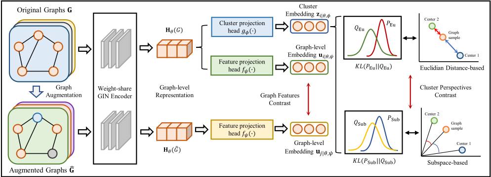
To answer this question, we propose a dual contrastive graph-level clustering (DCGLC) 1 in this paper. Figure 1 shows the network structure of DCGLC. Specifically, we leverage graph contrastive learning to enhance the effectiveness of graph-level representations by maximizing the consistency between positive sample pairs and inconsistency between negative sample pairs. Additionally, we introduce an explicit clustering objective into graph contrastive learning, which enables our model to be optimized for clustering and learns discriminative graph-level representations. Furthermore, we propose a contrastive mechanism to align clustering information from both the Euclidean-based and subspacebased cluster perspectives, where the former focuses on the geometric relationships between graphs while the latter captures their structural relationships. The proposed DCGLC encourages the incorporation of clustering information from different cluster perspectives and ensures the consistency of clustering assignment across them, which leads to more reliable clustering results. Besides, the graph-level features contrast, and cluster-perspective contrast can be mutually improved, facilitating the learning of cluster-friendly representations. We summarize the main contributions of this work as follows:
1 Code is available at: https://github.com/wownice333/DCGLC
- We propose DCGLC, an end-to-end clustering method unifying the optimization of graph contrastive learning with information integration of different cluster perspectives.
- We propose a cluster-perspective contrast mechanism to align the cluster information, which results in more reliable clustering assignments by considering both geometric and structural relationships between graphs.
- We demonstrate the effectiveness of DCGLC through extensive experiments on various types of graph benchmarks. Experimental results show that DCGLC outperforms stateof-the-art baselines in graph-level clustering.
2 RelatedWork
Deep Graph Clustering. Clustering [Xie et al., 2016; Zhang et al., 2022; Cai et al., 2022b; Fu et al., 2022; Yao et al., 2023; Zhang et al., 2023; Cai et al., 2024b] is a fundamental task in machine learning, and is crucial for realworld data analysis. With the upsurge of GNNs, deep graph clustering, especially node clustering, has received increasing attention and advancement in recent years. For instance, Wang et al. [2017] proposed a marginalized graph autoencoder, which leverages both structural information and intrinsic properties of graph data to learn effective node features for clustering. Bo et al. [2020] combined graph convolutional network (GCN) [Kipf and Welling, 2017; Chen et al., 2023b; Chen et al., 2023c] and an integrated clustering module to learn effective node features for graph clustering. Tu et al. [2021] proposed a dynamic fusion mechanism to fuse the structural information and attributes and further designed a triplet self-supervised strategy to produce reliable cluster assignment. As an emerging technique, GCL-based methods [Zhao et al., 2021; Pan and Kang, 2021; Liu et al., 2022; Liu et al., 2023b] are also widely studied. Zhao et al. [2021] proposed a contrastive node clustering framework that encourages the similarity of positive pairs generated by attribute masks, and the dissimilarity of negative pairs constituted from out-of-cluster samples. Pan and Kang [2021] leveraged contrastive learning to learn consensus representation from multiple views for node clustering. Liu et al. [2023b] proposed a contrastive graph clustering method that effectively mines hard samples in clustering. Despite remarkable advancements in node clustering, a substantial research gap persists in graph-level clustering, because measuring the relationships between graphs is more complicated than nodes within a single graph.
Graph Representation Learning. Graph representation learning [Xu et al., 2019; Wu et al., 2020; Sun et al., 2024] aims to learn graph-level representation by aggregating node features learned with powerful GNNs, and has witnessed remarkable progress. For example, Sun et al. [2020] maximized the mutual information between the global and substructural information of data to learn comprehensive graphlevel representations. You et al. [2020] proposed GraphCL, a graph augmentation mechanism to learn effective graph-level representations based on GCL [Zhu et al., 2021a] for graph classification. We also follow the graph augmentation strategies proposed in [You et al., 2020] in this study, e.g., node dropping, edge perturbation, attribute masking, and subgraph, to augment graph data. You et al. [2021] proposed JOAO to investigate the automatic graph augmentation mechanisms in GCL. However, the majority of existing approaches focused on classification tasks and still very limited efforts on graphlevel clustering. Besides, these approaches usually construct two-stage models, which poses a greater challenge for graphlevel clustering as no supervision information can be utilized.
3 ProposedMethod
3.1 ProblemFormulation
Let G = {G1, . . . , GN} be a set of N graphs and each graph is formulated as Gi = {Vi,Ei, {x(i) v }v∈Vi }, where Vi is the node set, Ei is the edge set, and x(i) v is the feature vector of node v on graph i. We regard the problem that aims to partition the graph set into C different groups without any supervision information as graph-level clustering, i.e., to let G = G(1) ∪G(2) · · · ∪G(C) , s.t. G(i) ∩G(j) = ∅, ∀i ̸= j. Different from the graph-level classification and node-level clustering [Wu et al., 2020], graph-level clustering is still a challenging task in machine learning and has rarely been studied [Xu et al., 2022] because measuring the relationships between graphs in an unsupervised setting is much more complex than: 1) nodes within a single graph and 2) in a supervised setting. Therefore, the important issue in graph-level clustering is the exploration of learning graph-level features that contain clustering information and are sufficiently discriminative. To this end, we propose to achieve graph-level clustering by solving the following general problem:
where ℓr|ψ(·) denotes the representation learning objective with the aim of learning effective graph-level features, and ℓc|ϕ(·) is the clustering objective with the aim of capturing cluster information. A GNN [Kipf and Welling, 2017; Zhou et al., 2020] based model hθ(·), which has become a paradigm for many graph-based tasks [Xu et al., 2019; Park and Neville, 2019; Bo et al., 2020], is generally leveraged to facilitate the learning of graph representations from graph data. In the following section, we will show how to solve (1) and achieve graph-level clustering through the joint training of learning effective graph-level representation and leveraging comprehensive cluster information.
3.2 Graph-Level Representation Contrast
We first present the representation learning module, where we attempt to explore the capability of GCL [Zhu et al., 2021a] in learning effective representation for graph-level clustering. As an emerging technique in graph representation learning, GCL-based methods surpass state-of-the-art mutual information (MI) maximization-based methods [Veliˇckovi´c et al., 2019; Sun et al., 2020] in many tasks such as graph-level classification [You et al., 2020; Zhu et al., 2021b] and nodelevel clustering [Zhao et al., 2021; Xia et al., 2022]. Specifically, given a graph Gj, the learned features of node i in the k-th GNN layer can be defined as:
where a(k) i denotes the aggregated neighbour features of node i, i.e., a(k) i = AGGREGATE(k) (h(k-1) v : v ∈ N(i)), and N(i) is the neighbor set of node i. COMBINE(·) indicates the operation of integrating the information between node i and its neighbours. In particular, the initial feature h(0) i = xi. Subsequently, the graph-level representation of graph Gj , i.e., Hθ(Gj), can be formulated as follows:
where hiθ denotes the concatenated features of node i among all K layers, i.e., hiθ = CONCAT({h(k) i }Kk=1 ), and nGj is the node numbers of graph Gj . Note that the READOUT(·) function (e.g., Sum, Average, or Max/Min) aims to integrate the local features within a graph to obtain graph-level features [Kipf and Welling, 2017; Xu et al., 2019], and we utilize the sum readout function in our implementation.
Given a graph G, we follow the graph augmentation strategy A in [You et al., 2020] to produce an augmented graph
ˆGi ∼ Ai( ˆGi|G). Note that a minibatch with Nb graphs in training will generate Nb augmented graphs. Therefore, the original graph Gi and its corresponding augmented graph ˆGi can be regarded as a positive pair in contrastive learning, and the combination of Gi with other augmented graphs { ˆGj, i ̸= j} can be regarded as negative pairs then. For each graph pair such as Gi and ˆGi, their graph-level representations Hθ(Gi), Hθ( ˆGi) can be obtained through a GNN encoder following Eqs. (2) and (3). Besides, the contrastive loss is generally calculated in the low-dimensional latent space, therefore a projection head fψ(·) is applied to project the graph-level representation Hθ(Gi), Hθ( ˆGi) into ui|θ,ψ and ˆui|θ,ψ. We use NT-Xent loss [Sohn, 2016] as the contrastive loss in this paper, the NT-Xent loss is to maximize the consistency among positive pairs and the inconsistency among negative pairs. It is worth noting that we do not further generate other negative samples, instead, we regard the other Nb - 1 augmented samples in a minibatch as negative samples. For the Nb graphs in a minibatch, we aim to align the learned graph-level representations from the two sets of augmented graphs, which can be achieved by minimizing
where sim(ui|θ,ψ, ˆuj|θ,ψ) = u⊤i|θ,ψ ˆuj|θ,ψ ∥ui|θ,ψ∥∥ˆuj|θ,ψ∥ denotes the cosine similarity function, and τ indicates the temperature parameter. The loss function aims to minimize the distance between feature vectors of the same samples while maximizing the distance between feature vectors of different samples, resulting in learning more discriminative graph-level representations. Apparently, an intuitive way to achieve graphlevel clustering is to directly perform k-means [Hartigan and Wong, 1979] or SC [Ng et al., 2001] in the learned graphlevel representation. However, there are two important issues in this solution:
- Graph-level representation learning and clustering are two separate processes without any explicitly defined clustering objective, which implies that they may fail to learn cluster-friendly graph-level representations. The empirical results in the experiment section also demonstrate that those two-stage clustering models, i.e., the simple combination of k-means/SC and graph kernels/graph representation learning, tend to be trivial solutions.
- The Euclidean-based (e.g., k-means) and subspace-based clustering (e.g., SC) criteria offer cluster information from different perspectives. Euclidean-based methods prioritize distance information between data, while subspace-based methods emphasize the angle information. Combining these two perspectives can potentially provide richer information for graph-level clustering.
3.3 Multiple Cluster Perspectives Contrast
To address these issues, we propose a cluster-perspective contrast approach that aligns clustering information derived from multiple perspectives, which also introduces an explicit clustering objective to guide the optimization. Specifically, inspired by [Xie et al., 2016; Cai et al., 2022a], we cluster from two perspectives by utilizing two clustering heads, i.e., 1) Euclidian-based and 2) subspace-based, respectively. It should be noted that the clustering task generally performs in a low-dimensional embedding space, therefore we further project the graph-level features Hθ(Gi) into the cluster embedding Zθ,ϕ with a projector gϕ(·) parameterized by ϕ. The Euclidian-based clustering head measures the discrepancy between the graph-level features and each cluster center with Euclidian distance, which can be defined as follows:
where µc is the c-th cluster center of C clusters in total and can be initialized by k-means. zi|θ,ϕ = gϕ(Hθ(Gi)) ∈ Rdz is the cluster embedding for graph Gi and dz is the dimension of cluster embedding. Another clustering head is based on subspace clustering, with the assumption that the data can be divided by several subspaces when they are projected into a low-dimensional embedding space. Consequently, the subspace-based clustering head can be formulated by the similarity between the cluster embedding and the defined subspace base as follows:
where D ∈ RCd×d is the subspace base with d-dimension. It can be initialized by the column space of clusters generated by performing k-means on Zθ,ϕ. ∥z⊤i|θ,ϕD(c) ∥2F quantifies the 'closeness' (cosine similarity) between the graph-level feature zi|θ,ϕ and the c-th subspace D(c) . η is the smooth parameter and is fixed as 2. Particularly, the subspace D should obey two rules: 1) ∥D(c) i ∥ = 1, i = 1, . . . , d, c = 1, . . . ,C; 2) ∥D(i)⊤D(j) ∥F ≤ τ, i ̸= j, τ → 0. In practice, we impose two constraints by:
where ⊙ denotes the Hadamard product, I is an identity matrix with the same size as D. O is a special matrix whose elements in each d-size block are 0 and the others are 1. The first term ensures each base vector is of unit length, preventing the value of max∥z⊤j|θ,ϕD(c) ∥2F from being zero. The second term encourages the subspace bases to be mutually orthogonal, which is critical for maintaining distinct and separate subspaces.
After defining the learnable cluster assignment QEu and QSub from the distance and subspace perspectives, we can further yield a refined assignment, e.g., PEu, defined as:
where Nb represents the number of graphs in a batch, and the effect of PEu is to emphasize the high-confidence assignments in QEu. Similarly, we can derive PSub from QSub via:
Algorithm 1 Training flows of DCGLC.
Input: Graph set G, number of clusters C, batch size Nb, learning rate α, total training epochs T .
Output: The clustering results C.
- 1: Initialize the parameters θ, ϕ, ψ and cluster centers µ;
- 2: while not converge do
- 3: for t = 1, 2, . . . , T do
- 4: Generate augmented graph set ˆG fromG;
- 5: Obtain graph representations Hθ(Gi) and Hθ( ˆGi) with Eq. (2) and (3);
- 6: Obtain the cluster embeddings Zi, and cluster assignments QEu and QSub with Eqs. (5) and (6);
- 7: Compute refined cluster assignments PEu and PSub via Eqs. (8) and (9);
- 8: end for
- 9: Compute the total loss with Eqs. (4), (7), (10), (11), and (12);
- 10: Back-propagation and update network parameters θ, ϕ, ψ, and the cluster centers µ;
- 11: end while
- 12: Compute final cluster assignment QEu and QSub;
- 13: Obtain the clustering labels with Eq. (13);
- 14: return The clustering results C.
Note that the refined assignments serve as the pseudo labels to provide guidance for the update of QEu and QSub, which can be optimized by minimizing the discrepancy between the cluster assignment distribution and the refined assignment distribution, i.e.:
where KL(·||·) denotes the Kullback-Leibler (KL) divergence between two distributions. As previously discussed, our objective is to learn reliable and consistent clustering assignments by incorporating more comprehensive cluster information from multiple cluster perspectives (i.e., Euclidianbased one denoted by QEu and subspace-based one denoted by QSub) for each graph. However, clustering from different perspectives may yield inconsistent results due to diverse evaluation criteria, which ultimately affects the consistency of clustering and leads to suboptimal clustering performance. To address this challenge, we propose a cluster-perspective contrast objective ℓc|θ,ϕ for the cluster information alignment of different perspectives, which is defined as follows:
where C denotes the number of clusters, and the definitions of τ and sim(·, ·) are same to Eq. (4). Notably, we also demonstrate that aligning different cluster perspectives outperforms solely utilizing a single clustering head with a comprehensive experiment via an ablation study (in Section 4.2).
3.4 Training Strategy
The two modules in the proposed method are jointly optimized by minimizing the following total objective function:
where λ and β are trade-off parameters that control the contributions of ℓc|θ,ϕ and ℓKL|θ,ϕ to the total loss. Compared to (1), we not only comprise a well-defined representation learning module and clustering module, but also incorporate cluster information from different cluster perspectives. The dual contrastive learning in graph-level feature pairs and multiple cluster perspectives allows us to obtain more reliable cluster assignments. More importantly, our approach stands out as an end-to-end graph-level clustering method that is able to produce clustering results directly from the network, eliminating the reliance on performing other clustering methods (e.g., k-means and SC) on the learned graph-level representations. The clustering results C for each graph can be obtain from the trained QEu and QSub by:
Algorithm 1 summarizes the detailed training flows of the proposed DCGLC.
3.5 Complexity Analysis
Here, we further theoretically analyze the time and space complexity for the proposed DCGLC method. Considering N graph with average n nodes and |E| edges per graph, the number of GIN layers and clusters are K and C, and the dimensions of nodes and each hidden layer are m and dh. We analyze the time and space complexity of DCGLC as follows:
- The time complexity of the first layer and the other layers in GIN are approximate O(Nn|E|mdh) and O(Nn|E|d2h ), where |E| typically can be ignored when the adjacency matrix is sparse. Besides, the time complexity of each cluster head is O(NKdhC). Therefore, the time complexity of DCGLC is O(Ndh(nm + (K - 1)ndh + 2KC)).
- Regarding space complexity, the GIN backbone in DCGLC needs to store the neighbor list and feature matrices of the entire graph to represent the graph structure. Thus the space complexity of these processes is O(Nn +N|E| +Nnm). Besides, the computation process of the GIN needs to store the intermediate results of each GIN layer. Thus the space complexity of this process for the GIN with K layers is O(Nndh(m+ (K - 1)dh)). The space complexity of the two cluster heads is O(NKdhC). Overall, the space complexity of DCGLC is O(Nn+N|E|+Nnm+Nndh(m+ (K - 1)dh) + 2NKdhC).
From the above discussion, we can observe that the time and space complexities of DCGLC are mainly associated with the number of nodes and graphs, i.e., n and N, which is competitive to GCL-based baselines such as GraphCL [You et al., 2020], JOAO [You et al., 2021], and GLCC [Ju et al., 2023].
3.6 Discussion with Previous Works
Numerous works have paved the way for this work, and we briefly discuss the connections between our work and them.
| Method | MUTAG | BZR | DD | IMDB-BINARY | ||||||||
|---|---|---|---|---|---|---|---|---|---|---|---|---|
| ACC | NMI | ARI | ACC | NMI | ARI | ACC | NMI | ARI | ACC | NMI | ARI | |
| SP | 72.87±0.00 | 10.24±0.00 | 15.95±0.00 | 79.51±0.00 | 4.13±0.00 | 3.97±0.00 | 58.83±0.00 | 0.43±0.00 | 0.14±0.00 | 53.95±1.15 | 6.52±1.69 | 0.66±0.36 |
| GK | 67.02±0.00 | 1.74±0.00 | 1.04±0.00 | 61.23±3.36 | 1.06±1.21 | 3.13±3.74 | 57.60±1.49 | 0.28±0.13 | -0.05±0.55 | 50.20±0.00 | 0.39±0.00 | 0.00±0.00 |
| RW | 77.65±0.00 | 30.81±0.00 | 30.26±0.00 | 64.69±0.00 | 0.00±0.00 | -0.15±0.00 | OM | OM | OM | 51.30±0.00 | 0.16±0.00 | 0.03±0.00 |
| WL | 73.40±0.00 | 14.50±0.00 | 21.20±0.00 | 75.56±0.00 | 0.50±0.00 | 3.76±0.00 | 58.57±0.00 | 0.13±0.00 | -0.05±0.00 | 51.24±0.53 | 0.69±0.79 | 0.06±0.05 |
| LT | 56.60±4.88 | 3.09±1.38 | -0.62±0.63 | 78.35±0.35 | 0.69±0.28 | 1.12±1.03 | OM | OM | OM | 51.20±0.00 | 1.61±0.00 | 0.05±0.00 |
| WL-OA | 67.55±0.00 | 19.64±0.00 | 11.40±0.00 | 69.63±0.00 | 5.60±0.00 | -8.67±0.00 | OM | OM | OM | 50.86±0.52 | 0.53±0.84 | 0.02±0.05 |
| InfoGraph+KM | 77.95±1.41 | 35.22±3.47 | 30.95±3.03 | 63.62±2.41 | 1.59±0.95 | 2.39±1.44 | 58.57±0.04 | 0.64±0.00 | -0.02±0.08 | 54.79±0.84 | 4.77±0.16 | 0.92±0.38 |
| InfoGraph+SC | 72.58±4.83 | 28.68±4.93 | 19.85±5.91 | 73.53±2.66 | 3.66±2.52 | 5.04±3.12 | 58.83±0.00 | 0.43±0.00 | 0.14±0.00 | 54.90±3.69 | 4.31±1.91 | 1.41±2.16 |
| GraphCL+KM | 77.07±1.21 | 35.69±2.83 | 28.99±2.65 | 71.43±4.09 | 1.04±0.77 | 3.07±1.03 | 58.02±0.04 | 0.67±0.00 | -0.33±0.03 | 54.66±0.13 | 5.16±0.19 | 0.83±0.02 |
| GraphCL+SC | 73.22±2.66 | 32.19±2.05 | 23.44±2.45 | 72.88±1.66 | 1.90±0.38 | 3.47±0.59 | 55.18±2.21 | 0.19±0.17 | 0.62±0.67 | 57.42±1.35 | 5.01±1.34 | 2.76±1.56 |
| JOAO+KM | 79.20±0.72 | 36.32±3.03 | 33.74±1.65 | 72.64±4.26 | 1.37±1.14 | 4.01±3.39 | 57.95±0.04 | 1.49±0.00 | -0.37±0.00 | 58.20±1.84 | 6.76±1.19 | 2.77±1.13 |
| JOAO+SC | 70.72±2.85 | 27.73±0.23 | 17.12±2.03 | 72.98±1.59 | 2.75±1.30 | 5.62±3.74 | 56.28±0.48 | 0.33±0.00 | 1.01±0.00 | 50.20±0.00 | 0.39±0.00 | 0.00±0.00 |
| GWF+KM | 66.94±7.68 | 12.46±9.31 | 13.32±10.53 | 53.00±0.31 | 3.42±0.45 | -0.76±0.05 | 53.35±1.91 | 0.08±0.01 | 0.24±0.24 | 56.93±2.65 | 1.58±0.96 | 2.07±1.31 |
| GWF+SC | 73.92±4.30 | 18.35±3.85 | 24.48±4.69 | 52.76±0.80 | 3.47±1.16 | -0.71±0.32 | 52.08±0.98 | 0.04±0.03 | -0.12±0.08 | 51.93±3.58 | 0.61±0.83 | 0.58±1.19 |
| GLCC | 71.99±3.08 | 13.18±6.93 | 16.89±8.28 | 63.62±9.79 | 1.18±0.60 | 1.12±0.97 | 60.70±0.00 | 2.40±0.00 | 2.30±0.00 | 66.50±0.00 | 8.10±0.00 | 10.60±0.00 |
| DCGLC | 86.70±0.87 | 42.55±3.18 | 53.02±3.10 | 81.73±0.00 | 13.57±0.00 | 18.27±0.00 | 74.93±1.22 | 18.44±1.42 | 24.72±2.32 | 66.50±2.37 | 9.16±2.09 | 11.03±2.72 |
The GCL methods, e.g., GraphCL [You et al., 2020] and JOAO [You et al., 2021], can be applied to graph-level clustering by performing k-means [Hartigan and Wong, 1979] or SC [Ng et al., 2001] on the learned representations. Compared with them, DCGLC allows graph-level representations for clustering tasks to be learned in an end-to-end manner, which guides graph representation learning with an explicitly defined clustering objective.
Some works also delved into end-to-end frameworks for jointly optimizing representation learning and clustering. For example, Xie et al. [2016] and Cai et al. [2022a] respectively investigated distance-based and subspace-based endto-end clustering models. However, they are not committed to clustering graph-level data and considered from a single cluster perspective. Ju et al. [2023] proposed a graph-level contrastive clustering method for learning clusters through instance-level and cluster-level contrast. However, the cluster-level contrast in [Ju et al., 2023; Li et al., 2021] focuses on aligning the logits prediction from the original and augmented data, which is quite different from ours. DCGLC introduces two cluster heads to explicitly define clusters, and focuses on leveraging comprehensive cluster information from different cluster perspectives to learn more reliable cluster assignments, which is substantiated by the ablation study results in Section 4.2.
4 Experiment
In this section, we conduct a series of evaluations to demonstrate the superiority of the proposed DCGLC.
4.1 Experimental Settings
Datasets. We consider three types of graph benchmark datasets to evaluate the clustering performance, including seven molecule datasets (MUTAG, BZR, PTC-MR, PTCMM, COX2, ER MD, and AIDS), three biological datasets (DD, PROTEINS and ENZYMES), and two social network datasets (IMDB-BINARY and REDDIT-MULTI-5K). Details of these benchmarks refer to Appendix A.
BaselineMethods. We compare the proposed method with several state-of-the-art baselines, which can be broadly classified into three categories including: 1) Graph Kernel: SP [Borgwardt and Kriegel, 2005], GK [Shervashidze et al., 2009], RW [Vishwanathan et al., 2010], WL [Shervashidze et al., 2011], LT [Johansson et al., 2014], WL-OA [Kriege et al., 2016], 2) Unsupervised Graph Representation Learning: InfoGraph [Sun et al., 2020], GraphCL [You et al., 2020], JOAO [You et al., 2021], 3) Graph-Level Clustering: GWF [Xu et al., 2022], GLCC [Ju et al., 2023]. Note that the network structure of InfoGraph [Sun et al., 2020], GraphCL [You et al., 2020], JOAO [You et al., 2021], and GLCC [Ju et al., 2023] are exactly the same as ours to guarantee a fair comparison.
Implementation Details. We employ a 4-layer GIN [Xu et al., 2019] as the backbone network for the proposed DCGLC, with the aggregated dimension set to 16. We utilize an MLPbased feature projection head and cluster projection head, with the dimension of the latent layer and the clustering embedding layer both set to 10. The number of clusters is set to the number of categories in the dataset, the batch size is fixed to 64, and the training epoch is set to 300 for all datasets. We use Adam as the optimizer and follow the setting in [You et al., 2021] to augment graphs automatically in each epoch. Other details and the setup of baseline models refer to Appendix B.
Evaluation Metrics. We use clustering accuracy (ACC), normalized mutual information (NMI), and adjusted rand index (ARI) as the evaluation metrics, and report the means and standard deviations of the three metrics based on 10 independent runs for each dataset.
4.2 Experimental Results
Comparison with State-of-the-art Baselines. Tables 12 present the experimental results on eight graph benchmarks from different data types (more results refer to Appendix C), where we compare the proposed DCGLC method with eleven state-of-the-art baselines. From this table, we have the following observations: 1) The proposed DCGLC
| Method | PTC-MR | PTC-MM | COX2 | ER MD | ||||||||
|---|---|---|---|---|---|---|---|---|---|---|---|---|
| ACC | NMI | ARI | ACC | NMI | ARI | ACC | NMI | ARI | ACC | NMI | ARI | |
| SP | 56.69±0.00 | 1.04±0.00 | 0.50±0.00 | 62.20±0.00 | 1.63±0.00 | 0.73±0.00 | 52.03±0.00 | 0.13±0.00 | 0.01±0.00 | 58.07±0.00 | 1.89±0.00 | -0.79±0.00 |
| GK | 56.40±0.00 | 1.32±0.00 | 0.31±0.00 | 62.20±0.00 | 1.63±0.00 | 0.73±0.00 | 66.17±0.00 | 0.02±0.00 | 0.08±0.17 | 57.85±0.00 | 2.18±0.00 | -0.91±0.00 |
| RW | 56.98±0.00 | 0.63±0.00 | 1.25±0.00 | 60.71±0.00 | 0.97±0.00 | 2.91±0.00 | 51.31±0.00 | 0.70±0.00 | -0.92±0.00 | 63.68±0.00 | 15.81±0.00 | 6.63±0.00 |
| WL | 52.91±0.00 | 0.23±0.00 | 0.05±0.00 | 62.20±0.00 | 1.50±0.00 | 3.87±0.00 | 50.54±0.00 | 0.51±0.00 | -0.40±0.00 | 61.43±0.00 | 2.35±0.00 | 2.30±0.00 |
| LT | 55.17±1.32 | 0.40±0.65 | 0.19±0.52 | 61.19±0.88 | 0.73±0.55 | 1.09±1.06 | 77.52±0.59 | 0.26±0.34 | 0.17±0.71 | 59.19±0.00 | 0.34±0.00 | -0.14±0.00 |
| WL-OA | 59.30±0.00 | 1.77±0.00 | 2.95±0.00 | 63.39±0.00 | 4.59±0.00 | 2.26±0.00 | 50.75±0.00 | 0.51±0.00 | -0.37±0.00 | 61.43±0.00 | 2.35±0.00 | 2.30±0.00 |
| InfoGraph+KM | 54.79±0.68 | 0.49±0.35 | 0.28±0.21 | 61.48±1.03 | 2.35±0.83 | 3.61±1.45 | 56.74±3.04 | 3.30±0.60 | 0.17±0.10 | 61.21±0.00 | 1.59±0.00 | 2.63±0.00 |
| InfoGraph+SC | 56.10±0.33 | 1.50±0.26 | 0.20±0.13 | 61.96±1.53 | 2.12±0.99 | 4.55±0.83 | 70.37±2.01 | 3.56±0.99 | 1.92±1.67 | 59.87±0.00 | 1.15±0.00 | 0.42±0.00 |
| GraphCL+KM | 54.33±0.76 | 1.15±0.55 | 0.16±0.29 | 58.93±0.74 | 0.27±0.15 | 0.60±0.14 | 68.88±0.59 | 1.05±0.21 | 0.44±0.57 | 60.99±0.00 | 1.50±0.00 | 3.35±0.00 |
| GraphCL+SC | 56.13±0.42 | 1.31±0.30 | 1.17±0.24 | 62.09±0.56 | 2.14±0.43 | 3.36±0.87 | 75.01±2.12 | 1.24±0.37 | 2.39±2.28 | 59.42±0.00 | 3.03±0.00 | 0.44±0.00 |
| JOAO+KM | 56.39±0.18 | 0.53±0.21 | 0.41±0.01 | 59.04±0.52 | 0.21±0.14 | 0.98±0.41 | 70.56±2.03 | 1.19±0.34 | 0.44±0.43 | 66.14±0.00 | 5.77±0.00 | 9.51±0.00 |
| JOAO+SC | 56.16±0.22 | 1.03±0.33 | 0.19±0.11 | 62.41±0.80 | 2.00±0.78 | 4.28±1.34 | 76.46±0.61 | 1.43±0.77 | 2.35±2.49 | 59.42±0.00 | 2.02±0.64 | 0.30±0.00 |
| GWF+KM | 56.33±3.52 | 1.09±0.88 | 1.65±1.50 | 53.37±3.18 | 0.30±0.37 | 0.38±1.09 | 57.60±4.11 | 1.50±0.13 | 2.08±1.80 | 51.94±1.87 | 0.27±0.56 | -0.07±0.27 |
| GWF+SC | 55.32±4.03 | 0.89±0.84 | 1.49±1.44 | 53.02±1.66 | 0.36±0.28 | 0.21±0.09 | 58.83±4.46 | 1.16±0.41 | 1.45±1.21 | 59.12±0.56 | 0.51±0.53 | -0.11±0.36 |
| GLCC | 56.10±3.29 | 1.21±0.63 | 1.38±1.15 | 61.61±0.24 | 0.63±0.41 | 1.24±1.38 | 77.37±1.11 | 0.02±0.03 | -0.30±0.42 | 61.21±1.28 | 5.24±1.38 | 4.61±1.16 |
DCGLC
59.98±1.11 2.60±0.89 3.66±0.92 65.48±0.24 4.32±0.70 7.34±0.15 78.63±0.16 3.05±0.82 5.42±3.15 66.95±0.18 10.12±0.88 11.29±0.25
Table 2: Clustering performance (mean ± std) on PTC-MR/MM, COX2, and ER MD (%). The results highlighted in bold and underlined
denote the best and runner-up performance respectively.

-100 -80 -60 -40 -20 0 20 40 60 80 100 -80 -60 -40 -20 0 20 40 60 80 100 0 1 method demonstrates significant superiority over state-of-theart graph kernels and graph-level clustering baselines. Particularly, compared to the GCL-based baselines, e.g., GraphCL, JOAO, and GLCC, the proposed DCGLC exhibits notable advantages across three different types of graph data. For example, on the molecule dataset MUTAG, DCGLC exceeds JOAO+KM with an improvement of 7.50%, 6.23%, and 19.28% in terms of ACC, NMI, and ARI. Besides, on the biology dataset DD, DCGLC also outperforms the runnerup GLCC by more than 14.00% across all metrics. These results clearly indicate that the dual contrastive mechanism in DCGLC can facilitate the learning of clustering-friendly graph representations. 2) Empirical results show that the one clustering perspective may not consistently yield superior performance. For instance, GWF+KM outperforms GWF+SC on PTC-MR and BZR, while the opposite is true for MUTAG and ER MD. This phenomenon is also observed in other state-of-the-art baselines, e.g., GraphCL, and JOAO. These observations suggest that different clustering perspectives reveal distinct information for clustering, which may exhibit different validity for various graph data. Besides, this also highlights the rationale for leveraging the cluster information from multiple clustering perspectives to promote graph-level clustering.
Visualization of Clustering Embedding. We employ tSNE [Van der Maaten and Hinton, 2008] to visualize the clustering embeddings to facilitate a more intuitive comparison. As shown in Figure 2, it is evident that InfoGraph yields a dis-
-100 -80 -60 -40 -20 0 20 40 60 80 100 -80 -60 -40 -20 0 20 40 60 80 0 1 organized result with no discernible clusters. While GraphCL and JOAO demonstrate better performance compared to InfoGraph, the samples of the same color are still widely dispersed. Besides, although GWF shows clearer boundaries between classes, the gap between the two classes is small, resulting in blurred clustering boundaries. Compared with them, the clustering structures of DCGLC are more compact, with different clusters more separated and samples from the same cluster being significantly closer in proximity. The improved compactness and separability of the clusters indicate the effectiveness of DCGLC in capturing and leveraging the underlying structure and relationships within the graph data for more accurate clustering.
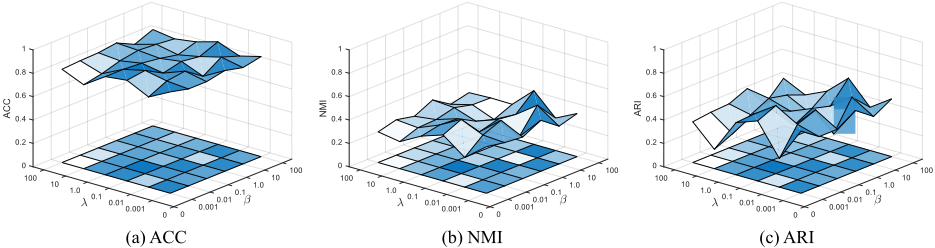
Impact of λ and β. We evaluate the impact of the variation of two hyper-parameters, λ, and β, on the clustering performance. Specifically, we conduct the parameter analysis by intentionally setting the values of λ and β within a broad range of [0.001, 100]. The results depicted in Figure 3 show the performance variations observed on MUTAG (more results refer to Appendix D). The empirical results reveal that excessively high values of λ generally lead to a negative impact on clustering performance. For instance, when λ is set to 100, the performance becomes unsatisfactory. Interestingly, our method demonstrates a remarkable insensitivity to changes in the value of β, as evidenced by its consistently stable performance across different values. Notably, the ARI tends to be more sensitive to variations in both λ and β. Overall, these findings collectively underscore the robustness and stability of DCGLC across a broad range of λ and β values.
Ablation Study. We conduct an ablation study to demonstrate the effectiveness of the proposed method and the rationale of integrating the cluster information from different perspectives. We construct three degradation variants for the proposed DCGLC, including:
- DCGLC v1: Drop out the cluster-perspective contrast component, and only consider the Euclidian-based clustering head and graph-level features contrast.
- DCGLC v2: Drop out the cluster-perspective contrast component, and only consider the subspace-based clustering head and graph-level features contrast.
- DCGLC v3: Drop out the graph-level features contrast component and only train under the guidance of clusterperspective contrast.
| Dataset | Metrics | DCGLC v1 | DCGLC v2 | DCGLC v3 | DCGLC |
|---|---|---|---|---|---|
| MUTAG | ACC NMI ARI | 78.94±5.64 26.04±12.07 32.85±14.16 | 78.99±3.11 23.85±5.42 32.95±6.86 | 84.47±1.48 41.62±2.11 47.17±5.17 | 86.70±0.87 42.55±3.18 53.02±3.10 |
| BZR | ACC NMI ARI | 79.48±1.11 5.78±4.32 11.41±5.46 | 80.74±0.80 9.31±3.01 12.35±4.68 | 79.16±0.79 8.05±1.62 15.24±4.66 | 81.73±0.00 13.57±0.00 18.27±0.00 |
| AIDS | ACC NMI ARI | 89.96±2.71 50.19±10.18 56.00±13.71 | 80.00±0.00 12.22±2.04 7.77±6.57 | 88.55±0.66 38.96±2.69 46.14±3.28 | 96.77±0.33 73.51±2.30 85.74±1.45 |
In Table 3, we thoroughly evaluate DCGLC in comparison to all degradation variants on three datasets (more results refer to Appendix E), revealing several key insights: 1) The Euclidean-based and subspace-based cluster perspectives each possess their own set of strengths and weaknesses. The former demonstrates superior performance on MUTAG, whereas the latter outperforms on BZR. This highlights the importance of considering different clustering perspectives, as their effectiveness can vary depending on the characteristics of graph data. 2) Relying solely on a single cluster perspective is insufficient for capturing comprehensive cluster information, as we observe consistent performance degradation DCGLC v1 and DCGLC v2. The results provide strong evidence for the validity of incorporating cluster information from different cluster perspectives in graph-level clustering. 3) The importance of graph-level features contrast is demonstrated from the results of DCGLC v3. Notably, removing this component leads to noticeable performance degradation, reaffirming its indispensable role in enabling the network to learn more effective graph representations.
5 Conclusion
In this paper, we proposed dual contrastive graph-level clustering (DCGLC). DCGLC leverages graph contrastive learning and introduces an explicit clustering objective to learn discriminative graph-level representations that are conducive to clustering. We highlight the importance of capturing comprehensive cluster information from multiple cluster perspectives to graph-level clustering, and propose a contrastive mechanism to align cluster information from different cluster perspectives. DCGLC is an end-to-end framework that integrates graph contrastive learning and cluster-perspective contrast, leading to a mutual enhancement during training. Extensive experiments on several popular graph benchmarks compared with state-of-the-art methods fully demonstrate the superiority of DCGLC. The main limitation of this work stems from the exploration of the graph augmentation mechanism beneficial for capturing better clustering structures, which is a promising research issue for future work.
Acknowledgments
This research is supported by the National Natural Science Foundation of China (Grants No.U21A20472, No.62276065, and No.62376236), and Shenzhen Research Institute of Big Data (Grant No.T00120210002).
Additionally, this research is supported by the National Research Foundation Singapore and DSO National Laboratories under the AI Singapore Programme (AISG Award No: AISG2-RP-2020-018). Any opinions, findings and conclusions or recommendations expressed in this material are those of the authors and do not reflect the views of National Research Foundation, Singapore.
Contribution Statement
Jinyu Cai and Yunhe Zhang contributed equally to this work as co-first authors.
@inproceedings{ijcai2024p417,
  title     = {Dual Contrastive Graph-Level Clustering with Multiple Cluster Perspectives Alignment},
  author    = {Cai, Jinyu and Zhang, Yunhe and Fan, Jicong and Du, Yali and Guo, Wenzhong},
  booktitle = {Proceedings of the Thirty-Third International Joint Conference on
               Artificial Intelligence, {IJCAI-24}},
  publisher = {International Joint Conferences on Artificial Intelligence Organization},
  editor    = {Kate Larson},
  pages     = {3770--3779},
  year      = {2024},
  month     = {8},
  note      = {Main Track},
  doi       = {10.24963/ijcai.2024/417},
  url       = {https://doi.org/10.24963/ijcai.2024/417},
}
TY - CPAPER TI - Dual Contrastive Graph-Level Clustering with Multiple Cluster Perspectives Alignment AU - Cai, Jinyu AU - Zhang, Yunhe AU - Fan, Jicong AU - Du, Yali AU - Guo, Wenzhong T2 - Proceedings of the Thirty-Third International Joint Conference on Artificial Intelligence, IJCAI-24 PB - International Joint Conferences on Artificial Intelligence Organization PY - 2024 SP - 3770 EP - 3779 DO - 10.24963/ijcai.2024/417 UR - https://doi.org/10.24963/ijcai.2024/417 ER -Copied
Machine-readable versions of this paper, for tools and AI agents:





