
Front-to-End Bidirectional Heuristic Search with Consistent Heuristics: Enumerating and Evaluating Algorithms and Bounds
Proceedings of the Thirty-Second International Joint Conference on Artificial Intelligence. Main Track. Pages 5631-5638.
https://doi.org/10.24963/ijcai.2023/625
Keywords
- Search: S: Heuristic search
Abstract
Recent research on bidirectional heuristic search (BiHS) is based on the must-expand pairs theory (MEP theory), which describes which pairs of nodes must be expanded during the search to guarantee the optimality of solutions. A separate line of research in BiHS has proposed algorithms that use lower bounds that are derived from consistent heuristics during search. This paper links these two directions, providing a comprehensive unifying view and showing that both existing and novel algorithms can be derived from the MEP theory. An extended set of bounds is formulated, encompassing both previously discovered bounds and new ones. Finally, the bounds are empirically evaluated by their contribution to the efficiency of the search
- [Alcázar et al., 2020] Vidal Alcázar, Patricia J. Riddle, and Mike Barley. A unifying view on individual bounds and heuristic inaccuracies in bidirectional search. In AAAI, pages 2327-2334. AAAI Press, 2020.
- [Alcázar, 2021] Vidal Alcázar. The consistent case in bidi- rectional search and a bucket-to-bucket algorithm as a middle ground between front-to-end and front-to-front. In ICAPS, pages 7-15. AAAI Press, 2021.
- [Chen et al., 2017] Jingwei Chen, Robert C. Holte, Sandra Zilles, and Nathan R. Sturtevant. Front-to-end bidirec- tional heuristic search with near-optimal node expansions. In IJCAI, pages 489-495. ijcai.org, 2017. IJCAI
- [Dechter and Pearl, 1985] Rina Dechter and Judea Pearl. Generalized best-first search strategies and the optimality of A*. J. ACM, 32(3):505-536, 1985.
- [Demetrescu et al., 2009] Camil Demetrescu, Andrew V Goldberg, and David S Johnson. The shortest path problem: Ninth DIMACS implementation challenge, vol- ume 74. American Mathematical Soc., 2009.
- [Eckerle et al., 2017] Jurgen Eckerle, Jingwei Chen, Nathan R. Sturtevant, Sandra Zilles, and Robert C. Holte. Sufficient conditions for node expansion in bidirectional heuristic search. In ICAPS, pages 79-87, 2017.
- [Felner et al., 2004] Ariel Felner, Richard E Korf, Ram Meshulam, and Robert C Holte. Compressing pattern databases. In National Conference on Artificial Intelli- gence (AAAI-04), pages 638-643, 2004.
- [Ford and Fulkerson, 1956] Lester Randolph Ford and Del- bert R Fulkerson. Maximal flow through a network. Cana- dian journal of Mathematics, 8:399-404, 1956.
- [Hart et al., 1968] Peter E. Hart, Nils J. Nilsson, and Bertram Raphael. A formal basis for the heuristic determination of minimum cost paths. IEEE Trans. Syst. Sci. Cybern., 4(2):100-107, 1968.
- [Helmert, 2010] Malte Helmert. Landmark heuristics for the pancake problem. In SoCS, pages 109-110. AAAI Press, 2010.
- [Kaindl and Kainz, 1997] Hermann Kaindl and Gerhard Kainz. Bidirectional heuristic search reconsidered. J. Artif. Intell. Res., 7:283-317, 1997.
- [Konig, 1931] Dénes Konig. Graphok es matrixok (hungar- ian)[graphs and matrices]. Matematikai és Fizikai Lapok, 38:116-119, 1931.
- [Korf, 1985] Richard E. Korf. Depth-first iterative- deepening: An optimal admissible tree search. Artif. In- tell., 27(1):97-109, 1985.
- [Papadimitriou and Steiglitz, 1998] Christos H Papadim- itriou and Kenneth Steiglitz. Combinatorial optimization: algorithms and complexity. Courier Corporation, 1998.
- [Pohl, 1971] Ira Pohl. Bi-directional search. In B. Meltzer and D. Michie, editors, Machine Intelligence, volume 6, pages 127-140. Edinburgh University Press, 1971.
- [Sadhukhan, 2012] Samir K. Sadhukhan. A new approach to bidirectional heuristic search using error functions. In CSI, 2012.
- [Sewell and Jacobson, 2021] Edward C. Sewell and Shel- don H. Jacobson. Dynamically improved bounds bidirec- tional search. Artif. Intell., 291:103405, 2021.
- [Shaham et al., 2017] Eshed Shaham, Ariel Felner, Jingwei Chen, and Nathan R. Sturtevant. The minimal set of states that must be expanded in a front-to-end bidirectional search. In SoCS, pages 82-90, 2017.
- [Shaham et al., 2018] Eshed Shaham, Ariel Felner, Nathan R. Sturtevant, and Jeffrey S. Rosenschein. Minimizing node expansions in bidirectional search with consistent heuristics. In SoCS, pages 81-98. AAAI Press, 2018.
- [Shperberg et al., 2019a] Shahaf S. Shperberg, Ariel Felner, Solomon Eyal Shimony, Nathan R. Sturtevant, and Avi Hayoun. Improving bidirectional heuristic search by bounds propagation. In SoCS, pages 106-114, 2019.
- [Shperberg et al., 2019b] Shahaf S. Shperberg, Ariel Felner, Nathan R. Sturtevant, Solomon Eyal Shimony, and Avi Hayoun. Enriching non-parametric bidirectional search al- gorithms. In AAAI, pages 2379-2386. AAAI Press, 2019.
- [Shperberg et al., 2021] Shahaf S. Shperberg, Steven Dani- shevski, Ariel Felner, and Nathan R. Sturtevant. Iterative- deepening bidirectional heuristic search with restricted memory. In ICAPS, pages 331-339. AAAI Press, 2021.
- [Sturtevant et al., 2020] Nathan R. Sturtevant, Shahaf S. Sh- perberg, Ariel Felner, and Jingwei Chen. Predicting the effectiveness of bidirectional heuristic search. In ICAPS, pages 281-290. AAAI Press, 2020.
- [Sturtevant, 2012] Nathan R. Sturtevant. Benchmarks for grid-based pathfinding. IEEE Trans. Comput. Intell. AI Games, 4(2):144-148, 2012.
References were extracted automatically from the PDF and may contain errors.
Full text extracted automatically from the PDF; figures, tables and equations may differ. The PDF is the version of record.
1 Introduction
Research on bidirectional heuristic search (BiHS) dates back to the late sixties. Recently, a new theory was developed for BiHS [Eckerle et al., 2017] that laid the foundation for a rich line of research in the area [Shaham et al., 2017; Shaham et al., 2018; Shperberg et al., 2019a; Sturtevant et al., 2020; Alc´azar et al., 2020; Alc´azar, 2021; Shperberg et al., 2021]. This theory of must-expand pairs (MEP) characterizes the set of forward- and backward- node pairs that must be expanded in order to prove solutions' optimality. Recent BiHS algorithms, such as NBS [Chen et al., 2017] and DVCBS [Shperberg et al., 2019b] utilize the MEP theory to reduce the search effort required to return optimal solutions.
This paper focuses on the case where the heuristic is known to be consistent. In this case, the conditions for which pairs of nodes must be expanded can be refined [Shaham et al., 2018], which reduces the number of MEPs. Thus, assuming consistency, these tighter conditions can potentially be exploited to further reduce the number of nodes expanded by BiHS algorithms. Algorithms like NBS and DVCBS, however, cannot be efficiently adapted to these tighter conditions, whose enforcement requires significantly more computational effort.
BiHS algorithms for the consistent heuristics case have also been developed. These algorithms utilize the information derived from heuristic consistency to maintain lower bounds (denoted search bounds) on solutions' cost, which in turn are used for speeding up the search [Kaindl and Kainz, 1997; Sadhukhan, 2012; Alc´azar et al., 2020; Sewell and Jacobson, 2021]. Fundamental questions include whether other bounds can be developed and how well they will perform.
To answer these questions, the conceptual gap between these algorithms and the MEP theory must be explored. This paper provides a unifying view that closes this gap. The contributions of this paper are : (1) A family of search bounds that can be directly derived from the MEP conditions. To our knowledge, this family includes all existing search bounds as well as novel search bounds. (2) A global algorithmic framework designed to exploit any subset of bounds; with a focus on exploiting single bounds for guiding the search. This framework encompasses previous search-bounds-based algorithms. (3) An experimental study on the effect of each bound and the behaviors of variants of the framework. We also compare the number of nodes expanded by these variants to the theoretical lower bound from the MEP theory, showing that existing algorithms are very close to the theoretical limits.
2 Definitions, Notations, and Background
In BiHS, the aim is to find a least-cost path, of cost C � , between start and goal in a given graph G. distpx, yq denotes the shortest distance between x and y, so dist pstart, goalq � C � . In some cases, the cost of the cheapest edge of the graph (denoted by ϵ) is available, otherwise, ϵ is assumed to be 0.
BiHS typically keeps two open lists, OpenF for the forward search (F), and OpenB for the backward search (B). Given a direction D (either F or B), we use fD, gD and hD to indicate f-, g-, and h-values in direction D. We use D to denote the direction that is opposite to D, and define fD , gD and hD symmetrically. This paper considers the two front-to-end heuristic functions [Kaindl and Kainz, 1997] hF psq and hBpsq which respectively estimate distps, goalq and distpstart, sq for all s P G. hF , is forward admissible iff hF psq / dist ps, goalq for all s in G and is forward consistent iff hF psq / distps, s1 q � hF ps1 q for all s and s1 in G. Backward admissibility and consistency are defined analogously.
In addition to the known g, h, and f functions, we define the following functions which are used throughout the paper:
(1) dDpnq � gDpnq � hD pnq, the difference between the actual cost in direction D of node n and its heuristic estimation; this indicates the heuristic error for node n.
(2) bDpnq � fDpnq � dDpnq. bDpnq adds the heuristic error dDpnq to fDpnq to indicate that the opposite search using hD pnq will underestimate by dDpnq.
(3) rf Dpnq � gDpnq � hDpnq, the reverse f-value [Alc´azar, 2021], a function that is similar to f, but which subtracts the heuristic instead of adding it.
(4) rdDpnq � gDpnq � hD pnq, the reverse d-value [Alc´azar, 2021], which adds the opposite heuristic instead of subtracting it. The term reverse for rf and rd was coined by Alc´azar et al. (2020). While the motivation behind rf and rd might seem unclear, they can be used as building blocks for some of the bounds on optimal solutions cost, as we show below.
Finally, we denote by xMinD the minimal x value in OpenD. For example, gMinD � minnPOpenD gDpnq, the minimal g-value in direction D. Additionally, tx, yuMinD is the minimal x � y value in OpenD, e.g., trf , duMin D � minnPOpenD trf Dpnq � dDpnqu. Likewise, tx, y, zuMinD is the minimal x � y � z value in direction D.
2.1 Must-Expand Nodes in Bidirectional Search
Any unidirectional heuristic search (UniHS) algorithm (meeting reasonable theoretical assumptions), that is guaranteed to find an optimal solution on every problem with an admissible heuristic, must expand all nodes n with fpnq � C � to prove the optimality of solutions when given a consistent heuristic [Dechter and Pearl, 1985].
The generalization of this theory to BiHS [Eckerle et al., 2017] showed that in BiHS the must expand attribute is defined on pairs of nodes pu, vq from the forward and backward frontiers (and not on a single node as in UniHS) as follows:
lbpu, vq �maxtfF puq, fBpvq, gF puq � gBpvq � ϵu (1) lbpu, vq is a lower bound on the cost of any path that can connect start and goal via u and v. In BiHS, a pair of nodes pu, vq is called a must-expand pair (denoted MEP) if lbpu, vq � C � . In a MEP at least one of u or v must be expanded. Otherwise, an algorithm that does not expand either u or v when lbpu, vq � C � might miss the optimal solution.
The set of MEPs can be reformulated as a bipartite graph, denoted as the Must-Expand Graph (GMX) [Chen et al., 2017]. For each state u P G, GMX includes a forward vertex uF and a backward vertex uB. For each pair of states u, v P G, there is an edge in GMX between uF and vB iff pu, vq is a MEP. Since each edge of GMX is a MEP and at least one node from each MEP must be expanded to ensure the optimality of the solution, it follows that any optimal algorithm must expand a vertex cover of GMX. Thus, the minimum number of node expansions required to guarantee the optimality of a solution for problem instance by BiHS is the size of the minimum vertex cover (denoted by MVC) of GMX. When consistency is not assumed, the MVC of GMX can be computed in linear time with respect to the number of nodes in the GMX [Shaham et al., 2017].
2.2 MEPs When Assuming a Consistent Heuristics
This paper focuses on the case where algorithms can assume that they are always given problem instances with a consistent heuristic (i.e., they do not need to return an optimal solution when given admissible heuristics that are not consistent).
We denote this as the consistency case, under which more information can be exploited and the aim is to develop algorithms that utilize this. For the consistency case, Shaham et al. (2018) introduced tighter lower bounds for pairs denoted lbCpu, vq (C for consistency):
All terms in the max expression are lower bounds on distpu, vq and can thus be added to gF puq � gBpvq. ϵ (term 2c) is a trivial lower bound, term 2a is derived from the definition of a forward-consistent heuristic: hF puq / distpu, vq � hF pvq øæ hF puq � hF pvq / distpu, vq, and term 2b is derived analogously from the definition of backward consistency. 1 lbCpu, vq induces a new MEP definition, denoted as MEPC. Since lbCpu, vq / lbpu, vq for every pair of nodes u, v, the number of MEPCs is smaller than or equal to the number of MEPs for any given problem instance.
Finally, for undirected graphs, lbCpu, vq can be further tightened resulting in lbCUpu, vq (U for undirected):
Both Equations 2 and 3 can be used for defining corresponding GMX graphs, however, in these cases the MVC can no longer be computed in linear time [Shaham et al., 2018].
2.3 NBS and DVCBS
Near-Optimal Bidirectional Search (NBS) [Chen et al., 2017] is a prominent algorithm based on the MEP theory. At every expansion cycle, NBS chooses a pair of nodes u, v with a minimal lbpu, vq (denoted as LB) among all pairs in the open lists, and expands both nodes. This approach is based on the 2-factor approximation of minimal vertex covers [Papadimitriou and Steiglitz, 1998]. Thus, NBS is guaranteed to expand a vertex cover of GMX whose size is at most 2 � |MV C|. To find a pair with minimal lb value, NBS uses two-level priority queues in each direction, a waiting queue which stores all nodes n with fDpnq ¡ LB, sorted by f, and ready queue which stores all nodes n with fDpnq / LB sorted by g. These data structures enable NBS to only expand MEPs, while maintaining amortized insertion and deletion time of logpnq, where n is the number of frontier nodes.
Dynamic Vertex Cover Bidirectional Search (DVCBS) [Shperberg et al., 2019b] is a competitor to NBS. DVCBS constructs a partial, dynamic GMX (denoted DGMX) based on the nodes currently in OPEN, finds an MVC of DGMX, and expands all nodes in this MVC. DVCBS is unbounded in the worst case, but empirically outperforms NBS on average. DVCBS computes the MVC of DGMX by bucketing nodes with the same fD- and gD-values and solving a weighted MVC problem in time that is linear in the number of buckets.
1 Equation 1 for lbpu, vq includes terms for fF puq and fBpvq. These terms are redundant in lbCpu, vq, as gF puq�gBpvq�hF puq� hF pvq � fF puq�dBpvq ¡ fF puq, and for fBpvq using term 2b.
An issue arises when attempting to adapt NBS and DVCBS to the consistency case. Although NBS can be defined for lbC (Equation 2) and lbCU (Equation 3), its two-level priority queue is no longer suitable for efficiently identifying a pair with the minimum lbC (or lbCU) value. Similarly, DVCBS can no longer achieve a linear-time MVC of DGMX. In an effort to develop an efficient algorithm for the consistency case, Alc´azar (2021) introduced a method called bucket-to-bucket (BTB). This scheme involves grouping nodes into buckets that share the same gD, hD, hD values. Using these buckets, both NBS and DVCBS can be applied using lbC (or lbCU). However, each expansion cycle of a bucket requires a computational overhead that is quadratic in the number of buckets. While the number of buckets may be small in certain domains, in general, there could be an arbitrary number of buckets. As a result, the quadratic runtime for every expansion cycle can become impractical (e.g., in road maps or grids).
2.4 Search Bounds, DIBBS/BAE*, and DBBS
We use the term search bounds [Alc´azar et al., 2020] to denote all lower bounds on the solution cost that can be computed during the search. We classify the search bounds into three categories. (1) Global bounds provide a lower bound on the cost of every solution from start to goal. These bounds can be used as termination conditions; when the incumbent solution has a cost that equals the bound then it is optimal. (2) Individual-node bounds bound the cost of every solution from start to goal that passes through a given node n (e.g. lbpnq). (3) Pair bounds bound the cost of paths from start to goal that passes through a given pair of nodes u, v, where u P OpenF and v P OpenB (e.g., lbpu, vq).
Several search bounds have been used in the heuristic search literature. In UniHS the minimal f-value in the open list, fMin, is a global bound on the cost of any solution. This f -bound is commonly used in the termination conditions of many algorithms (both unidirectional and bidirectional). Similarly, in BiHS, fMinF and fMinB are global bounds. Another bound in BiHS is the g-bound� gMinF +gMinB �ϵ.
For the consistency case, other search bounds have been proposed. Kaindl and Kainz (1997) proposed adding heuristic errors (defined as dDpnq above), of direction D, to fvalues of the opposite direction D. In particular, they defined the following individual-node bounds KKAddDpnq � fDpnq � dMinD and symmetrically, KKMaxDpnq � dDpnq � fMinD . Note that these node bounds can be transformed to be global bounds by taking the minimal f- and dvalues from both directions as follows: KKAdd � fMinD� dMinD and KKMax � dMinD � fMinD . A lower bound b1 is said to dominate another lower bound b2 iff b1 ¥ b2 . Since fMinD � dMinD ¥ fMinF then KKAdd dominates fMinF . Similarly, KKMax dominates fMinB. Another global bound is the foundation of two identical algorithms, BAE* [Sadhukhan, 2012] and DIBBS [Sewell and Jacobson, 2021], which expand nodes with minimal b-value. They introduce a new global bound, b-bound� pbMinF � bMinBq{2, and terminate when a solution is found with cost � b-bound.
Alc´azar (2021) combined the KK bounds, the g-bound, and the b-bound together to improve their individual performance. In this context, a node n is defined as expandable iff n P argminn1 POpenD pmaxtfDpn1 q�dMinD , dDpn1 q� fMinD , pbDpn1 q � bMinD q{2, gDpuq � gMin D � ϵu. For an undirected graph, two more bounds were introduced: rfMinF � rdMinB (forward rc (reverse consistent)) and rdMinF � rfMinB (backward rc). The minimal values in the open lists, which are used for defining the global search bounds, can be computed with respect to the set of expandable nodes. This creates a fixpoint computation in which the minimal values in the open lists are updated based on the set of expandable nodes, and the set of expandable nodes is updated based on the updated minimal values in the open lists until convergence is reached. The DBBS algorithm [Alc´azar, 2021] performs this fixpoint computation to find tighter bounds, and thus expand fewer nodes during the search. This process, however, is computationally expensive.
3 Deriving Bounds from the MEP Theory
In this section, we introduce a unifying view for the consistency case and draw a connection between lbC (Equation 2) and all existing search bounds (presented in Section 2.4). In addition, we show that additional search bounds can be derived from lbC and even more bounds can be derived when also considering undirected graphs (lbCU , Equation 3).
A first step towards a unifying view was taken by Alc´azar (2021) who observed that taking each element in the max term of Equation 2 (2a, 2b, and 2c) individually, can derive the KKAdd, KKMax , and g-bound, correspondingly. For example, for term 2a, gF puq�gBpvq�hF puq�hF pvq � fF puq � dBpvq ¥ fMinF � dMinB � KKAdd . However, the method of taking individual elements of the max term is limited and cannot be used for producing other bounds, e.g., the b-bound. We now provide a general way to produce more bounds from the max term. In fact, any max function over a set of elements S can be bounded from below as follows:
where PpSq is the power set of S (i.e., the average of the elements of any subset of S is always a lower bound of the maximal element in S). Using this rule, the max expression in Equation 2 can be lower-bounded by different subsets S1 of the terms inside (i.e., 2a, 2b, and 2c). For example, when taking S1 � t2a, 2bu, we get the b-bound (B4 below):
By considering all subsets S1 of terms 2a, 2b, and 2c, and for a node n by replacing the value xDpnq with the minimal x-value in OpenD, xMinD, as was demonstrated above (for 2a and for 2a, 2b), we get the following global bounds:
B1: fMinF �dMinB (KKAdd), when S1 � t2au
B2: dMinF � fMinB (KKMax), when S1 � t2bu
B3: gMinF � gMinB � ϵ (g-bound), when S1 � t2cu
B4: bMinF�bMinB 2 (b-bound), when S1 � t2a, 2bu
B5: tf,guMinF�td,guMinB�ϵ 2 , when S1 � t2a, 2cu
B6: td,guMinF�tf,guMinB�ϵ 2 , when S1 � t2b, 2cu
The derivation of each of the bounds tB1, . . . ,B7u can be done similarly to the two examples presented above.
We note that substantial work was done to individually prove each of the previously proposed bounds (e.g., [Kaindl and Kainz, 1997; Sewell and Jacobson, 2021]), whereas the derivation of these bounds from the MEP theory is straightforward. Finally, note that individual-node bounds that correspond to each of the above global bounds tB1, . . . ,B7u can be derived from the MEP theory as well. This is done by replacing the value of xDpnq with the minimal x value in OpenD (xMinD) in one of the two directions instead of the two directions, as was done in the derivations above. For example, the last step in the KKAdd derivation above pB1q becomes fF puq � dBpvq ¥ fF puq � dMinB.
3.1 Bounds for Undirected Graphs
For undirected graphs, we derive lower bounds from lbCU instead of lbC. Since terms 2a, 2b, and 2c are identical to 3a, 3b, and 3c, the above seven bounds tB1, . . . , B7u are also valid for for lbCU. Nevertheless, additional bounds for the max expression can be derived from terms 3d and 3e. At first glance, it might seem that there are 31 possible search bounds for lbCU (corresponding to the 31 possible subsets of terms 3a to 3e excluding H). However, note that terms 3a and 3d cancel each other (3a � 3d � hF puq � hF pvq � hF pvq � hF puq � 0). Thus, all subsets S1 that contain both term 3a and term 3d are dominated either by S1 zt3au or by S1 zt3du (which are also valid subsets of S), and can be ignored. The same argument holds for terms 3b and 3e. Thus, we are left with only 17 bounds that are not dominated by other bounds. The resulting (additional) bounds and their respective subsets of terms are as follows:
B8: rfMinF � rdMinB (forward rc), when S1 � t3du
B9: rdMinF � rfMinB (backward rc), when S1 � t3eu
B10: tf,rduMinF�trf ,duMinB 2 , when S1 � t3a, 3eu
B11: trf ,duMinF�tf,rduMinB 2 , when S1 � t3b, 3du
B12: trf ,guMinF�trd,guMinB�ϵ 2 , when S1 � t3c, 3du
B13: trd,guMinF�trf ,guMinB�ϵ 2 , when S1 � t3c, 3eu
B14: trf ,rduMinF�trf ,rduMinB 2 , when S1 � t3d, 3eu
The above set of bounds (tB1, . . . , B7u and tB1, . . . , B17u for Equation 2 and Equation 3 (respectively) are all the possible bounds that can be produced when approximating the max term in the equations using Equation 4. Other lower bounds would require to bound the max terms in different ways (possibly using a convex combination) or using other methods altogether. Another possibility for generating new bounds is to introduce additional assumptions. For instance, as shown by Alc´azar et al. (2020), if the greatest common denominator among the cost of all non-zero-cost edges, denoted as ι, is known, it can be used to tighten the bounds further. For each bound Bi from the above set of bounds, we can use ιr Bi ι s as a possibly tighter version of Bi. So, in unit-edge-cost graphs, all of the above bounds can be rounded up.
4 Using the Bounds within Algorithms
We now turn to the practical aspects of the proposed bounds. We describe a general BiHS algorithmic framework for the consistency case, presented in Algorithm 1, and show how to utilize information from the bounds in this framework. There are three decisions that define BiHS algorithms: (1) deciding when to terminate the search, (2) choosing which node to expand from a given direction, and (3) choosing the direction from which the next node will be expanded. Each of these can utilize information from the bounds.
4.1 Termination Condition
Each global bound Bi can be used to prove that the incumbent solution is optimal, i.e., when a solution is found with cost � Bi the algorithm can terminate. Naturally, when there are several lower bounds, their maximum is the tightest lower bound among them and can be used as a termination condition. The advantage of using several bounds is that if we have the optimal solution U (with cost C � ) in hand, we can halt faster: once Bi � C � for any of the available global bound Bi. The tradeoff is the overhead of maintaining and consulting several bounds. In addition, the bounds can be computed either with the (computationally expensive) fixpoint computation, as in DBBS, or without it.
4.2 ChoosingWhich Node to Expand
The decision of which node in OpenD to expand next (i.e., what priority function to use) is at the heart of any search algorithm. Since each global bound Bi is essentially a termination condition, expanding nodes that will cause Bi to increase as early as possible would likely result in earlier termination. For example, A* [Hart et al., 1968] terminates when a solution is found whose cost equals the minimal f-value in OpenF (fMinF ). Consequently, A* expands a node n with fpnq � fMinF , as this expansion policy is targeted at increasing the f-bound. Similarly, BAE* and DIBBS used the b-bound as a termination condition and thus expand nodes n with minimal bDpnq value. In a similar manner, expansion policies can be defined to target each of the above bounds. For example, the expansion policy that focuses on increasing KKAdd (bound B1) expands a node n with minimal fF pnqvalue or the node m with minimal dBpmq, depending on the chosen direction D. In general, each of our bounds has a
Algorithm 1: BiHS General Algorithmic Framework
1 U - 8, LB - ComputeLowerBoundpq 2 while OpenF �H^OpenB �H^U ¡ LB do 3 D-ChooseDirectionpq 4 n-ChooseNodepDq 5 Expandpn,Dq // update U 6 LB -ComputeLowerBoundpq 7 return Uterm to minimize from the forward side and a term to minimize from the backward side, and we choose to expand a node whose bound equals the relevant Min term according to the chosen direction D.
When several global bounds are used, we need to choose which bound to target. Many policies are possible; we describe two of them that we used in our experiments:
Targeting the max. This policy targets the bound which has the maximal value among all bounds, Bmax . The motivation here is that if we manage to raise this bound by expanding nodes, then we have a higher chance that the incumbent solution U will have costpUq � Bmax , and the algorithm can terminate. Thus, we choose to expand a node n in a given direction D whose individual bound Bmax pnq � Bmax .
Targeting the bound with the smallest span. Given a global bound B, we define spanpBq to be the number of nodes n with an individual-node bound Bpnq � B. Let Bss be the global bound with the smallest span in the set of bounds. This policy chooses to expand a node n whose individual bound Bsspnq � Bss . The intuition for this policy is to focus on the bound that would require the smallest effort to increase. 2
4.3 ChoosingWhich Side to Expand
Finally, we deal with the decision of whether to expand a node from OpenF or OpenB at each step. To this end, we explore three policies: alternating, cardinality criterion [Pohl, 1971], and a new policy called fastest bound increase (FBI). The alternating policy switches between forward and backward sides, while the cardinality criterion selects the side with the smallest open list. FBI aims to achieve the fastest increase in a specific bound Bi by comparing the spans of Bi in OpenF and OpenB and choosing the direction with the smaller span. For policies targeting the maximal bound or minimal span, FBI calculates Bmax or Bss for both directions and selects the side with the smallest span.
5 Empirical Evaluation
The main purpose of the empirical evaluation is to assess the different bounds. To this end, we implemented a targeted bound algorithm for each of the 17 bounds, denoted as TBi for all 1 / i / 17. In TBi we use all 17 bounds for termination (Line 3 in Algorithm 1), but only the targeted bound Bi for choosing which node to expand (Line 5 in Algorithm 1).
2 This is a greedy computation based on the current state of the open lists, as new nodes with the same Bss-values can be generated.
A secondary objective is to compare the performance of the new algorithms with notable existing algorithms and to determine when each algorithm should be used. For this, we evaluated BAE*, which uses only the b-bound for both node expansion and as the termination condition (related to TB4 that expands nodes with minimal b-value, but terminates using all the bounds). We evaluated both Pohl's cardinality criterion (denoted (p)) and alternating (denoted (a)) as sideselection policies (Line 4 in Algorithm 1) for BAE* and the TBi algorithms. We also experimented with A* and reverse A* (denoted as rA*), which performs the search from goal to start as representatives of UniHS algorithms. In addition, for determining the effect of the consistency assumption on the search we experimented with NBS and DVCBS, which assume heuristic admissibility, but not consistency. Finally, to study the effect of the fixpoint computation on the new bounds, we ran DBBS, which uses the original four global bounds, as well as DBBS all , which uses all 17 global bounds. For the DBBS variants, we evaluate the node-expansion policy that targets the b-bound (as in [Alc´azar et al., 2020]), and the new node-expansion policies, max and smallest span. For side-selection policies, we use (a), (p), and (FBI).
Finally, we calculated the theoretical lower bound on the number of expansions required to guarantee the optimality of solutions. To this end, we compute and report the MVC of GMX using lb (Equation. 1), in which only heuristic admissibility is assumed, as well as the MVC of GMXCU (defined according to lbCU, Equation. 3), in which the consistency is also assumed. This is the first time that GMXCU has been computed in the BiHS literature. To compute the MVC, we constructed GMXCU post facto (by collecting all nodes with fDpnq � C � to buckets), reduced the problem to a max-flow problem (K¨onig's theorem [Konig, 1931]), and ran the Ford-Fulkerson algorithm [Ford and Fulkerson, 1956] to find the maximal flow, which is equal to the MVC of GMXCU. The difference between the MVC and the actual number of nodes expanded by the evaluated algorithms indicates whether new BiHS algorithms that assume consistency should be developed (if there is a significant gap between them) or the focus should be turned elsewhere.
5.1 Experimental Settings
Domains. We experimented on five domains: (1) 50 14pancake puzzle instances with the GAP heuristic [Helmert, 2010]. To get a range of heuristic strengths, we also used the GAP-n heuristics (for 1 / n / 6) where the n smallest pancakes are left out of the heuristic computation. (2) The standard 100 instances of the 15 puzzle problem (STP) [Korf, 1985] using the Manhattan distance (MD) heuristic. (3) Grid-based pathfinding using octile distance as a heuristic and 1.5 cost for diagonal edges: 156 maps from Dragon Age Origins (DAO) [Sturtevant, 2012], each with different start and goal points (a total of 3149 instances); (4) 50 instances of the 12-disk 4-peg Towers of Hanoi (TOH) problem with (10+2), (8+4) and (6+6) additive PDBs [Felner et al., 2004]; and, (5) 100 random road map instances [Demetrescu et al., 2009] on the map of Colorado, using the Euclidean distance divided by the maximum speed as a heuristic.
| ToH - 12 | DAO | Road Maps | STP | ||||||||||
|---|---|---|---|---|---|---|---|---|---|---|---|---|---|
| PDB (10+2) | PDB (8+4) | PDB (6+6) | Octile | Dist{Speed max | MD | ||||||||
| Algorithm | ⁄ C � | � C � | ⁄ C � | � C � | ⁄ C � | � C � | ⁄ C � | � C � | ⁄ C � | � C � | ⁄ C � | � C � | |
| Admissible | A* rA* NBS DVCBS MVC(GMX) | 276K 123K 230K 232K | 276K 123K 230K 232K 123K | 1,926K 622K 647K 619K | 1,925K 620K 645K 609K 557K | 3,268K 1,064K 682K 663K | 3,239K 1,033K 662K 635K 624K | 5,406 5,342 6,873 5,545 | 5,322 5,267 6,556 5,151 4,290 | 127K 126K 96K 126K | 127K 126K 96K 126K 78K | 15,550K 11,144K 12,556K 10,930K | 14,700K 10,956K 11,739K 10,720K 9,267K |
| MVC(GMXCU) | 41K | 174K | 363K | N/A | N/A | 1,308K | |||||||
| BAE*(a) | 47K | 46K 53K | 187K 204K | 186K 204K | 383K 424K | 382K 423K | 6,718 7,081 | 6,668 6,940 | 67K 70K | 67K 70K | 2,707K | 2,700K 12,953K | |
| Consistent | TB1(a) TB2(a) TB3(a) TB4(a) TB5(a) TB6(a) TB7(a) DBBS all b DBBS all all | 54K 69K 648K 47K 263K 282K 170K 48K 49K 48K 48K 59K 50K | 69K 622K 46K 262K 277K 165K 46K 48K 47K 46K | 240K 662K 187K 386K 412K 315K 189K 200K 194K | 240K 660K 186K 382K 406K 308K 186K 197K 192K 186K | 435K 683K 383K 515K 513K 458K 383K 407K 395K 383K 549K | 435K 664K 382K 509K 512K 455K 379K 400K 393K 379K | 7,150 10,275 6,706 9,213 9,221 8,562 6,105 5,649 | 7,018 8,654 6,483 7,955 8,021 7,563 5,829 5,369 4,935 5,827 | 72K 119K 67K 96K 96K 86K N/A N/A N/A N/A | 72K 119K 67K 96K 96K 86K N/A N/A N/A N/A | 13,404K 10,815K N/A 2,707K N/A N/A 13,448K 2,262K 2,521K 2,027K 2,262K | 10,677K N/A 2,700K N/A N/A 13,275K 1,701K 1,761K 1,677K |
| DBBSb(a) | |||||||||||||
| DBBSmax(FBI) DBBSss(FBI) (a) max (FBI) | 189K | 5,374 6,104 | 1,701K | ||||||||||
| 55K | 236K | 233K | 527K | 5,648 | 5,367 | N/A | N/A | 3,057K | 2,208K | ||||
| DBBS ss (FBI) | 48K | 195K | 194K | 398K | 397K | 5,595 | 5,181 | N/A | N/A | 2,054K | 1,705K | ||
| GAP | GAP-2 | GAP-4 | ||||
|---|---|---|---|---|---|---|
| Algorithm | � C � | ⁄ C � | � C � | ⁄ C � | � C � | ⁄ C � |
| Admissible A* rA* | 72 77 | 46 52 | 351K 350K | 348K 349K | 47,289K 48,323K | N/A N/A |
| NBS DVCBS MVC(GMX) | 148 209 | 66 47 39 | 123K 85K | 122K 84K | 1,433K 977K | 1,433K 899K |
| MVC(GMXCU) BAE*(a) TB1(a) | 90 136 | 37 66 86 | 15K 78K | 82K 6,711 11K | 469K | N/A N/A |
| TB2(a) TB3(a) TB4(a) TB5(a) TB6(a) | 149 484K 90 27K 26K | 100 120K 16K 16K | 81K 15K 150K 153K | 78K 79K | 1,623K 469K | 1,623K 465K 634K |
| Consistent | 114 329 | 57 46 | 142K 33K 8,801 | 465K 5,492K 6,036K | ||
| 104 114 | 43 57 | 1,508K 35K 10K 18K 8,545 10K | 1,508K 11K 133K 10K 7,678 | 5,581K 6,178K 674K 741K 301K 277K | 658K 282K 272K 378K 230K | |
| 2,724 | 2,073 | |||||
| 447K 232K | ||||||
| DBBSss(FBI) DBBS all b (a) all | 66 | |||||
| TB7(a) | ||||||
| DBBSb(a) | ||||||
| DBBSmax(FBI) | ||||||
| 8,801 | 274K | 269K | ||||
| DBBS max (FBI) | 307 | 46 | 21K | 11K | 394K | 310K |
| DBBS all (FBI) | 104 | 43 | 8,410 | 7,562 | 223K | 219K |
| ss | ||||||
Metrics. For each algorithm, we report the average number of node expansions required to terminate (denoted as / C � ). In addition, we report the average number of necessary expansions required to prove optimality (denoted as � C � ), i.e., the number of nodes expanded until LB has reached C � .
Hardware. We ran the experiment on an 82-machine cluster. Each combination of algorithm and problem instance had a memory limit of 128GB and a time limit of 24 hours. When algorithms failed to solve some problems due to time or memory limits, the results are reported as N/A.
5.2 Results
Due to space limitations, only the results for bounds 1-7 (without the undirected graphs assumption) are included, as bounds 8-17 were shown to be weak. Moreover, results for the cardinality (p) side-selection policy are not reported, as there were no significant differences compared to the alternating policy. The results for ToH, DAO, road maps, and STP appear in Table 1 and for the pancake problem in Table 2.
Comparison to the MVC of the GMXs
In ToH, STP, and pancake the MVC of GMX is significantly larger than the MVC of GMXCU (by a factor of 3 for ToH, 7 for STP, and 8-15 for pancake, except for GAP, which is very accurate). This shows that the consistency assumption significantly reduces the number of necessary expansions in these domains. In road maps and DAO the MVC of GMXCU was too costly to compute due to large solution costs and many unique buckets. Nonetheless, the performance of the algorithms that only assume admissibility compared to algorithms that also make the consistency assumption hint that the MVC of GMX and GMXCU have a similar size in DAO, while the MVC of GMXCU is smaller in road maps by a small margin.
Comparison of Node Expansions
In ToH and road maps, BAE* had the best performance among all algorithms, similar to DBBS all b (except for road maps, in which the DBBS variants could not complete execution due to the 24h runtime limit). Moreover, the difference between the number of nodes expanded by BAE* and the MVC of GMXCU is very small (5 � 10%). Therefore, BAE* is very close to optimal, and no other algorithm (UniHS or BiHS) will be able to significantly improve over it. Finally, we see that the performance of BAE* is identical to TB4, which means that the b-bound was always the tightest and never benefited from the other termination criteria.
In STP, BAE* and TB4 were the best among the bounds that do not make use of fixpoint computation, improving over A*, rA*, NBS and DVCBS by a factor ¡ 4. Here too, the additional stopping criteria of TB4 did not improve the performance over BAE*. The DBBS variants, which perform the fixpoint computation, improved over BAE* by approximately
25%, where the best-performing variant was DBBSss(FBI). In fact, DBBSss(FBI) expands only 28% more nodes than the MVC of GMXCU before raising LB to C � . Thus, there is only a small margin left for improvement in STP as well.
In contrast to ToH, STP, and road maps, BAE* does not performwell on DAO. In this domain, rA* required the least expansions to return a solution, and DBBSss(FBI) required only a few additional expansions (/ C � ), and fewer necessary expansions (� C � ). Notably, the additional termination conditions of TB4 show a (small) improvement over BAE*, which means that the b-bound is not always dominating in DAO, even when the node-expansion policy only targets b.
Finally, in pancake (Table 2), we see a slightly different trend. A* is the best-performing algorithm for GAP, which is a very accurate heuristic, though DBBSss(FBI) required fewer necessary expansions. Among the algorithms that do not perform the fixpoint computation, BAE* had the best performance on GAP-1 and GAP-2, while TB7 (which also uses the g-value of nodes, as well as ϵ) had a better performance (by up to a factor of 2) on GAP-3 to GAP-5, which are weaker heuristics. When also considering algorithms that perform the fixpoint computation, the new DBBS all ss (FBI) has the best performance for GAP-1 to GAP-5, improving over the best non-fixpoint algorithm by up to 40%, and getting close to the theoretical bound (MVC), with a difference of at most 15%.
The Effect of Bounds throughout the Search
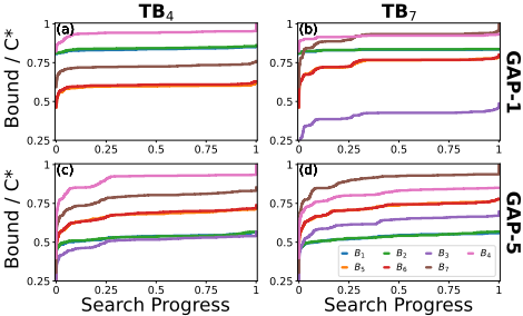
We now turn to analyze the effect of the TBi variants for different values of i on the value of all used bound throughout the search. Figure 1 shows the average value of each of the 7 bounds (as a fraction of C � ) during the search on the pancake domain using two targeted bounds, TB4 (b-bound, left) and TB7 (right), and two heuristics, GAP-1 (top) and GAP-5 (bottom). The bound on top in each plot is the dominating bound, and the search terminates when this dominating bound equals C � . Figures 1c and 1d show that on GAP-5, the bound that is targeted is the one with the highest value throughout the search, indicating that the targeted-bound policy achieves its purpose of rapidly increasing the bound of interest. However, Figure 1b shows that when one of the non-targeted bounds is significantly better than the targeted bound, the non-targeted bound might still have the highest value during the search.
| STP | DAO | |||
|---|---|---|---|---|
| Algorithm | Time (s) | n{s | Time (ms) | n ⁄ms |
| A* | 55.42 | 281K | 2.28 | 2371.12 |
| BAE*(a) | 10.07 | 269K | 4.08 | 1646.61 |
| TB4(a) | 59.99 | 45K | 87.69 | 76.48 |
| DBBSb(a) | 34.85 | 65K | 2,390.74 | 2.55 |
Runtime Analysis
Table 3 shows a focused report of the runtime for representative algorithms and problem instances. We used DAO and STP as polynomial and exponential representative domains, respectively. We aim to answer the following questions: (1) What is the overhead of using all bounds for termination compared to using a single bound? (2) What is the overhead of the fixpoint computation? and (3) How does the overhead of the BiHS algorithms compare to A*? The results show that BAE* is between 6 and 20 times faster than TB4, due to the overhead required to maintain all other bounds (a sorted vector of pointers for each bound). This suggests that TB4 should never be used, as its greater runtime overhead does not justify the small reduction in node expansions. As for the second question, the runtime of DBBS (i.e., the fixpoint computation) in DAO (polynomial domain) is several orders of magnitude smaller than other algorithms, while in STP (exponential domain) DBBS is only four times slower in terms of node expansions per second. Nonetheless, even in STP we see that BAE* is faster than DBBS in terms of total runtime, despite expanding more nodes. Finally, we see that A* is only slightly faster than BAE* in terms of expansions per second, thus the total runtime of the two algorithms mostly depends on their respective number of expansions.
As a general guideline, based on the empirical evaluation, BAE* should be the default algorithm to use for the consistency case, as it strikes a good balance between node expansions and runtime across different domains and heuristics. For weaker heuristics (e.g., as seen in GAP-4), we suggest using a targeted-bound algorithm that uses only B7. While in some domains the DBBS variants expand the least number of nodes, the overhead of the fixpoint computation is not justified in terms of total runtime.
6 Summary and Conclusions
This paper drew a connection between the MEP theory and the existing search bounds, showing that all bounds can be directly derived from the theory. Furthermore, we introduced a set of 17 search bounds, both existing and novel. Algorithms that target each of these bounds were developed and evaluated, showing that the b-bound is the most informative bound for most domains, but another bound (B7, which uses both b and g) is better for weak heuristics. In addition, the DBBS variants often expand the smallest number of nodes, but they incur an expensive computation overhead that always resulted in larger runtime. Finally, we compared the actual expansions by algorithms to the optimal number of necessary expansions, showing that there is not much room for further improvement. So, the focus on BiHS research can now move away from devising more algorithms for the consistency case.
Acknowledgements
This research was supported by the US-Israel Binational Science Foundation (BSF) grant no. 2021643. This work was also funded by the Canada CIFAR AI Chairs Program. We acknowledge the support of the Natural Sciences and Engineering Research Council of Canada (NSERC).
@inproceedings{ijcai2023p625,
  title     = {Front-to-End Bidirectional Heuristic Search with Consistent Heuristics: Enumerating and Evaluating Algorithms and Bounds},
  author    = {Siag, Lior and Shperberg, Shahaf and Felner, Ariel and Sturtevant, Nathan},
  booktitle = {Proceedings of the Thirty-Second International Joint Conference on
               Artificial Intelligence, {IJCAI-23}},
  publisher = {International Joint Conferences on Artificial Intelligence Organization},
  editor    = {Edith Elkind},
  pages     = {5631--5638},
  year      = {2023},
  month     = {8},
  note      = {Main Track},
  doi       = {10.24963/ijcai.2023/625},
  url       = {https://doi.org/10.24963/ijcai.2023/625},
}
TY - CPAPER TI - Front-to-End Bidirectional Heuristic Search with Consistent Heuristics: Enumerating and Evaluating Algorithms and Bounds AU - Siag, Lior AU - Shperberg, Shahaf AU - Felner, Ariel AU - Sturtevant, Nathan T2 - Proceedings of the Thirty-Second International Joint Conference on Artificial Intelligence, IJCAI-23 PB - International Joint Conferences on Artificial Intelligence Organization PY - 2023 SP - 5631 EP - 5638 DO - 10.24963/ijcai.2023/625 UR - https://doi.org/10.24963/ijcai.2023/625 ER -Copied
Machine-readable versions of this paper, for tools and AI agents:





