
Self-Recover: Forecasting Block Maxima in Time Series from Predictors with Disparate Temporal Coverage Using Self-Supervised Learning
Proceedings of the Thirty-Second International Joint Conference on Artificial Intelligence. Main Track. Pages 3723-3731.
https://doi.org/10.24963/ijcai.2023/414
Keywords
- Machine Learning: ML: Self-supervised Learning
- Machine Learning: ML: Representation learning
- Machine Learning: ML: Time series and data streams
Abstract
Forecasting the block maxima of a future time window is a challenging task due to the difficulty in inferring the tail distribution of a target variable. As the historical observations alone may not be sufficient to train robust models to predict the block maxima, domain-driven process models are often available in many scientific domains to supplement the observation data and improve the forecast accuracy. Unfortunately, coupling the historical observations with process model outputs is a challenge due to their disparate temporal coverage. This paper presents Self-Recover, a deep learning framework to predict the block maxima of a time window by employing self-supervised learning to address the varying temporal data coverage problem. Specifically Self-Recover uses a combination of contrastive and generative self-supervised learning schemes along with a denoising autoencoder to impute the missing values. The framework also combines representations of the historical observations with process model outputs via a residual learning approach and learns the generalized extreme value (GEV) distribution characterizing the block maxima values. This enables the framework to reliably estimate the block maxima of each time window along with its confidence interval. Extensive experiments on real-world datasets demonstrate the superiority of Self-Recover compared to other state-of-the-art forecasting methods.
- [Aliabadi et al., 2020] Majid Moradi Aliabadi, Hajar Emami, Ming Dong, and Yinlun Huang. Attention-based recurrent neural network for multistep-ahead predic- tion of process performance. Computers & Chemical Engineering, 140:106931, 2020.
- [Che et al., 2018] Zhengping Che, Sanjay Purushotham, Kyunghyun Cho, David Sontag, and Yan Liu. Recurrent neural networks for multivariate time series with missing values. Scientific reports, 8(1):1-12, 2018.
- [Chen et al., 2020] Ting Chen, Simon Kornblith, Moham- mad Norouzi, and Geoffrey Hinton. A simple framework for contrastive learning of visual representations. In Inter- national Conference on Machine Learning, pages 1597- 1607, 2020.
- [Coles et al., 2001] Stuart Coles, Joanna Bawa, Lesley Tren- ner, and Pat Dorazio. An introduction to statistical model- ing of extreme values, volume 208. Springer, 2001.
- [Ding et al., 2019] Daizong Ding, Mi Zhang, Xudong Pan, Min Yang, and Xiangnan He. Modeling extreme events in time series prediction. In Proceedings of the 25th ACM SIGKDD International Conference on Knowledge Discov- ery & Data Mining, pages 1114-1122, 2019.
- [Ericsson et al., 2022] Linus Ericsson, Henry Gouk, Chen Change Loy, and Timothy M Hospedales. Self- supervised representation learning: Introduction, ad- vances, and challenges. IEEE Signal Processing Magazine, 39(3):42-62, 2022.
- [Fawaz et al., 2020] Hassan Ismail Fawaz, Benjamin Lu- cas, Germain Forestier, Charlotte Pelletier, Daniel F Schmidt, Jonathan Weber, Geoffrey I Webb, Lhassane Idoumghar, Pierre-Alain Muller, and Franc ¸ois Petitjean. Inceptiontime: Finding alexnet for time series classifica- tion. Data Mining and Knowledge Discovery, 34(6):1936- 1962, 2020.
- [Galib et al., 2022] Asadullah Hill Galib, Andrew McDon- ald, Tyler Wilson, Lifeng Luo, and Pang-Ning Tan. Deep- extrema: A deep learning approach for forecasting block maxima in time series data. In Proceedings of the Thirty- First International Joint Conference on Artificial Intel- ligence, IJCAI-22, pages 2980-2986. International Joint Conferences on Artificial Intelligence, 7 2022. IJCAI
- [Hochreiter, 1998] Sepp Hochreiter. The vanishing gradient problem during learning recurrent neural nets and problem solutions. International Journal of Uncertainty, Fuzziness and Knowledge-Based Systems, 6(02):107-116, 1998.
- [Jaiswal et al., 2020] Ashish Jaiswal, Ashwin Ramesh Babu, Mohammad Zaki Zadeh, Debapriya Banerjee, and Fillia Makedon. A survey on contrastive self-supervised learn- ing. Technologies, 9(1):2, 2020.
- [Kingma and Ba, 2014] Diederik P Kingma and Jimmy Ba. Adam: A method for stochastic optimization. arXiv preprint arXiv:1412.6980, 2014.
- [Landsea and Franklin, 2013] Christopher W Landsea and James L Franklin. Atlantic hurricane database uncer- tainty and presentation of a new database format. Monthly Weather Review, 141(10):3576-3592, 2013.
- [Laptev et al., 2017] Nikolay Laptev, Jason Yosinski, Li Er- ran Li, and Slawek Smyl. Time-series extreme event fore- casting with neural networks at uber. In International con- ference on machine learning, volume 34, pages 1-5, 2017.
- [McDonald et al., 2022] Andrew McDonald, Pang-Ning Tan, and Lifeng Luo. Comet flows: Towards generative modeling of multivariate extremes and tail dependence. In Lud De Raedt, editor, Proceedings of the Thirty-First International Joint Conference on Artificial Intelli- gence, IJCAI-22, pages 3328-3334. International Joint Conferences on Artificial Intelligence, 7 2022. IJCAI
- [Peng et al., 2018] Chenglei Peng, Yang Li, Yao Yu, Yu Zhou, and Sidan Du. Multi-step-ahead host load pre- diction with gru based encoder-decoder in cloud comput- ing. In 2018 10th International Conference on Knowledge and Smart Technology (KST), pages 186-191, 2018.
- [Polson and Sokolov, 2020] Michael Polson and Vadim Sokolov. Deep learning for energy markets. Applied Stochastic Models in Business and Industry, 36(1):195- 209, 2020.
- [Sagheer and Kotb, 2019] Alaa Sagheer and Mostafa Kotb. Time series forecasting of petroleum production using deep lstm recurrent networks. Neurocomputing, 323:203- 213, 2019.
- [Vaswani et al., 2017] Ashish Vaswani, Noam Shazeer, Niki Parmar, Jakob Uszkoreit, Llion Jones, Aidan N Gomez, Łukasz Kaiser, and Illia Polosukhin. Attention is all you need. Advances in Neural Information Processing Sys- tems, 30, 2017.
- [Vincent et al., 2010] Pascal Vincent, Hugo Larochelle, Is- abelle Lajoie, Yoshua Bengio, Pierre-Antoine Manzagol, and Léon Bottou. Stacked denoising autoencoders: Learn- ing useful representations in a deep network with a lo- cal denoising criterion. Journal of Machine Learning Re- search, 11(12), 2010.
- [Wang et al., 2020] Bin Wang, Tianrui Li, Zheng Yan, Guangquan Zhang, and Jie Lu. Deeppipe: A distribution- free uncertainty quantification approach for time series forecasting. Neurocomputing, 397:11-19, 2020.
- [Wilson et al., 2022] Tyler Wilson, Pang-Ning Tan, and Lifeng Luo. DeepGPD: A Deep Learning Approach for Modeling Geospatio-Temporal Extreme Events. In Pro- ceedings of the 36th AAAI Conference on Artificial Intelli- gence, 2022.
- [Winkler et al., 2011] Julie A Winkler, Galina S Guentchev, Malgorzata Liszewska, and Pang-Ning Tan. Climate sce- nario development and applications for local/regional cli- mate change impact assessments: An overview for the non-climate scientist: Part ii: Considerations when using climate change scenarios. Geography Compass, 5(6):301- 328, 2011.
References were extracted automatically from the PDF and may contain errors.
Full text extracted automatically from the PDF; figures, tables and equations may differ. The PDF is the version of record.
1 Introduction
Forecasting the block maxima of a future time window is important as it enables us to anticipate the worst-case scenario expected to occur within the forecast period. In recent years, deep learning [Sagheer and Kotb, 2019; Laptev et al., 2017; Peng et al., 2018; Vaswani et al., 2017; Aliabadi et al., 2020] has become increasingly popular for time series forecasting due to their capacity to learn complex nonlinear relationships in data. However, since these methods are mostly designed to predict the conditional mean of the target variable rather than its tail distribution, they may not be effective at predicting the block maxima values. This has led to considerable interest in incorporating sound statistical principles from extreme value theory (EVT) into the deep learning formulation [Galib et al., 2022; McDonald et al., 2022; Wilson et al., 2022; Ding et al., 2019; Polson and Sokolov, 2020].
Forecasting block maxima is an inherently hard problem due to the limited availability of extreme values in historical data. Towards this end, process-based models have been developed in many scientific domains to simulate the future based on current understanding of the physical processes driving the changes observed in the system. For example, general circulation models (GCMs) are widely-used processbased models for generating forecasts of the future climate condition under varying greenhouse gas emission scenarios. Such model-based forecasts can be used as domain-informed predictors to complement the historical data and enhance the accuracy of time series forecasting models. However, integrating such model-based forecasts with historical observations is a challenge due to their disparate temporal coverageFor example, long-term historical records of the climate are dating back before the 20th century, whereas most of the archived scenarios of GCM runs are only available starting from mid-20th century since scenario development is timeconsuming and costly [Winkler et al., 2011]. The missing values in model-based forecasts can significantly impede training of accurate models [Che et al., 2018].
Self-supervised learning [Ericsson et al., 2022; Jaiswal et al., 2020] offers a possible solution to remedy this problem by extracting useful features from the available time series and using the information for missing value imputation. While self-supervised learning has demonstrated remarkable success in applications such as image and natural language processing, its utility in imputing missing values in time series has remained relatively unexplored. In this paper, we present a self-supervised learning framework called Self-Recover to enable accurate forecasts of the block maxima using both historical observations and modelbased forecasts. Specifically, a combination of contrastive and generative self-supervised learning methods along with a denoising autoencoder are used to impute missing values in the model-based forecasts. Self-Recover also employs a residual learning approach to combine representations of the historical and process model predictors so they can be used by downstream models for block maxima prediction. In this work, we employ DeepExtrema [Galib et al., 2022] as our downstream model due to its ability to simultaneously infer parameters of the generalized extreme value (GEV) distribution that characterizes the distribution of block maxima values and to accurately predict the block maxima of each time window along with its confidence interval.
In summary, the main contributions of the paper are:
- We present a novel framework, Self-Recover, to simultaneously recover the missing values present in the outputs of process-based models and to accurately forecast the block maxima of a future time window.
- We propose a self-supervised learning approach to impute both random and structured missing values present in a time series by integrating contrastive and generative learning schemes with a denoising autoencoder.
- We present a residual technique to combine the representations from historical and model-based forecasts and show that it is better than simple concatenation.
- We perform extensive experiments on real-world data to demonstrate the effectiveness of Self-Recover compared to state-of-the-art time series forecasting methods.
2 Preliminaries
2.1 Problem Statement
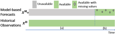
Consider a time series dataset that is partitioned into a set of potentially overlapping time windows, {w1,w2, · · · ,wn}. Each window wi is defined by a time interval [ti -α, ti +β], where [ti - α, ti] denotes the historical period of the time window and [ti + 1, ti + β] denotes the forecast period. Let {zH t }Tt=1 be the time series associated with the target variable to be predicted and {zM t }Tt=ts be the time series associated with the output forecasts generated by a set of m processbased models. For each time window [t - α, t + β], we denote xHt = (zH t-α, zH t-α+1 , · · · , zH t ) ∈ Rα+1 as the historical predictors, xM0 t = (zM t+1 , zM t+2 , · · · , zM t+β ) ∈ Rm×β as the model-based predictors, and yt = maxτ∈{1,··· ,β} z(H) t+τ ∈ R as the true block maxima of the forecast period. Note that the model-based predictors xM◦ t can be partially or completely missing for the given time window, as illustrated in Figure 1.
Our first objective is to impute the missing values in the model-based predictors (xM0 t ) using the historical predictors
(xHt ) available in [t - α, t]. To do so, we will train a data imputation model fimpute : Rα+1 → Rm×β to obtain the complete set of model-based forecasts, xMf t = fimpute(xHt ). Our second objective is to predict the block maxima value (yt) of the future period [t+1, t+β] using both the historical predictors (xHt ) in [t-α, t] and the (possibly imputed) modelbased predictors (xMf t ) in [t + 1, t + β]. This is achieved by training a model fforecast : Rα+1 ×Rm×β → R to predict the block maxima value, ˆ yt = fforecast(xHt , xMf t ), along with its upper and lower quantiles, ˆ yU and ˆ yL, respectively.
2.2 DeepExtrema Framework
The DeepExtrema framework [Galib et al., 2022] is designed to predict the block maxima of a time window by incorporating the following GEV distribution [Coles et al., 2001] into the training of deep neural networks (DNNs):
where the GEV parameters define the location (µ), scale (σ) and shape (ξ) of the distribution. The GEV parameters are constrained to satisfy the following conditions:
DeepExtrema uses a DNN to predict the block maxima value of a forecast period while simultaneously learning the parameters of its GEV distribution. The learned parameters can be used to estimate the forecast uncertainties by computing the pth quantile of the GEV distribution, yp, as follows:
Given a training set consisting of n block maxima values, {y1, y2, · · · , yn}, DeepExtrema is trained to minimize the mean-square error of the block maxima prediction as well as the following negative log-likelihood function to ensure its predictions are consistent with the GEV distribution:
DeepExtrema reformulates the GEV constraints given in (2) and reparameterizes the DNN output accordingly to ensure that the constraints are enforced during training. It further uses a model bias offset mechanism to ensure that the DNN output preserves the GEV constraints even when it is randomly initialized. The model bias offset mechanism would first compute the bias introduced by the randomly initialized network and then performs bias correction to mitigate its effect in subsequent training epochs. This strategy of debiasing the DNN outputs guarantees that the GEV parameters estimated by the DNN would satisfy the regularity conditions at all times even if the DNN was not properly initialized.
3 Proposed Self-Recover Framework
Self-Recover extends the DeepExtrema framework [Galib et al., 2022] to enable the incorporation of both historical observations and model-based forecasts as predictors for its block maxima prediction. Figure 2 presents a schematic diagram of the framework. Given the historical observations, Self-Recover initially imputes the structured missing values present in the model-based forecasts by employing a combination of contrastive and generative self-supervised learning schemes. A denoising autoencoder (DAE) is then used to impute values that are missing at random. Self-Recover implements two DNNs, consisting of stacked bidirectional LSTMs with a fully connected network, to learn the feature representations of the historical and model-based predictors separately. The learned model-based representation, hM , can be viewed as a residual term to be added to the representation of the historical observations, hH . The combined representation of hT and hM is then presented to a downstream model for block maxima prediction. Motivated by the DeepExtrema framework, the downstream forecasting module of Self-Recover works as follows:
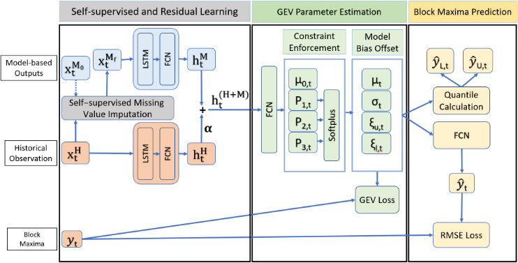
Equation (4) specifies a DNN model for estimating the GEV parameters governing the distribution of block maxima values based on the input predictors. The estimated GEV parameters are then used to forecast the block maxima along with its upper and lower quantiles according to Equation (5).
3.1 Self-Supervised Imputation for Handling the Disparate Temporal Coverage Problem
To deal with the difference in temporal coverage of the model-based forecasts and historical observations, Self-Recover employs a combination of self-supervised imputation approaches shown in Figure 3.
First, a contrastive learning approach is used to derive the feature representation of the historical observations. Contrastive learning [Jaiswal et al., 2020] is a method for learning representations from unlabeled data by comparing different augmented versions of the same data sample. In the context of time series, this would involve training a DNN with pairs of time series, where each pair is either a positive example (two similar time series) or a negative example (two dissimilar time series). The DNN is trained to identify features that will distinguish between the positive and negative examples.
Given the historical time series xHt of a window wt, a data augmentation step is initially performed to produce two perturbed time series, (xH1,t , xH2,t ). All other samples from the same mini-batch are treated as negative examples when paired with xHt . We evaluated different strategies for data augmentation, including jittering, scaling, and flipping but found jittering to perform the best. The augmented time series are then presented to an encoder-decoder network to generate the initial model-based forecasts xM′ t as follows:
The intermediate embedding (zH t ) of the encoder is projected to a lower-dimensional space using a projection head g(·), i.e., cHt = g(zH t ). To ensure that the projected vectors cHt are similar for closely related samples, a contrastive loss is calculated to measure the similarity between two projected vectors. The contrastive loss for positive examples containing pairs of augmented time series generated from the same xHt should be smaller than that for negative examples.
The encoder-decoder network given in (6) is trained to generate an initial model-based forecasts (xM′ t ) from the historical observations (xHt ). Although the initially generated forecasts are complete, i.e., have no missing values, they may not be consistent with the true model-based forecasts xM0 t . Thus, they need to be calibrated to ensure their consistency with the available ground truth model-based forecast values. Since the ground truth forecasts may also contain missing values, a denoising autoencoder (DAE) [Vincent et al., 2010] is used. DAE is a type of autoencoder designed to reconstruct the original values from a corrupted input by learning a representation that is robust to noise. ADAE imputes values that are missing at random by treating them as noise and training an autoencoder to recover their original values.
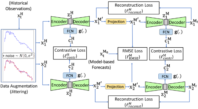
To apply the DAE, missing values are introduced as noise to perturb the complete model-based forecasts xM′ t . There are two cases to consider here. First, if its corresponding ground truth model-based forecasts xM0 t have missing values, then the same missing values are injected into xM′ t . Second, if no ground truth model-based forecasts are available or if there are no missing values in xM0 t , then the missing values are introduced randomly into xM′ t . In both cases, a corrupted model-based forecasts, xM′o t , is obtained from xM′ t , as shown in Figure 3. The DAE is trained to reconstruct the complete model-based forecasts xM′ t from the corrupted version xM′o t .
The embedding zM t generated by the DAE's encoder is also projected to a lower-dimensional space using a projection head g′ (·) to obtain a projected vector cMt = g′ (zM t ). Once again, to ensure that the projected vectors are similar for similar input samples, a contrastive loss is introduced for cMt . Finally, if the ground truth model-based forecasts xM0 t are available, a root-mean-square error (RMSE) loss is computed to ensure that the corrupted model-based forecasts xM′0 t remains close to xM0 t . The output of the DAE (xMf t ) is a complete set of model-based forecasts to be used for representation learning, as shown in Figure 2.
3.2 Optimization of Self-Supervised Imputation
The self-supervised imputation framework shown in Figure 3 is trained to minimize the following objective function:
where γ1, γ2, and γ3 are user-specified hyperparameters. The objective function LSSL comprises of a weighted sum of the contrastive loss for historical observations and model-based forecasts as well as the reconstruction and RMSE losses.
For contrastive learning, Self-Recover adopts the NTXent (Normalized Temperature-scaled Cross Entropy) loss function used in [Chen et al., 2020]. The contrastive loss associated with the latent historical (ℓHcontrast ) and model-based
(ℓMcontrast ) feature representations are defined as follows:
where P corresponding to the set of positive examples and sim(c1, c2) is the cosine similarity between two vectors.
The following reconstruction loss is used to train the DAE:
where xM′ t,i is the initially generated model-based forecasts by the encoder-decoder network and xMf t,i is the output of the DAE for the i-th sample.
Finally, the RMSE loss between ground truth model-based forecasts, xM0 t,i , and projected model-based forecasts xM′0 t,i is:
Self-Recover optimizes the objective function given in Equation (7) in two phases. During the first phase, it starts by training using only samples from the time period (b) shown in Figure 1, where both historical and model-based forecasts are available. After several hundred training epochs, it will proceed to the second phase in which the network is trained using samples from both time periods (a) and (b). The optimization is carried out this way to take advantage of the samples from time period (b) which have ground truth values available. The ground truth enables us to compute the RMSE loss and allows the network to converge faster towards the right local minima solution. Samples from the time period (a) will not contribute to the RMSE loss given in Equation (10) since they have no corresponding ground truth model-based forecasts.
3.3 Temporal Representation Learning
The self-supervised imputation step described in the previous subsection enables all the structured and random missing values in the model-based forecasts to be imputed. This allows Self-Recover to learn the temporal representations of both historical predictors (hHt ) as well as the model-based forecasts (hHt ) using a combination of stacked bi-directional LSTM and fully connected networks. The next step is to combine the two learned representations (hHt and hMt ) so they can be used to infer the GEV distribution parameters. One way to do this is to concatenate them together into a single representation, but this would increase its dimensionality and number of DNN parameters to be estimated in subsequent layers. Such a DNN is harder to train and is more susceptible to the vanishing gradient problem [Hochreiter, 1998].
Alternatively, the learned representation of the historical predictors (hHt ) can be regarded as a first-order approximation of the features. The learned representation from modelbased forecasts (hMt ) can be viewed as a residual (correction) factor to refine the representation error in hHt :
where α is a scalar hyperparameter for the residual weight.
We investigate the effectiveness of both approachessimple concatenation versus residual learning-and compare their relative performance in terms of effectiveness (forecast accuracy) and efficiency (convergence rate). As will be shown in our experiments, although the accuracy of both approaches is quite comparable, Self-Recover achieves faster convergence when using the residual learning approach compared to simple concatenation.
3.4 Incorporating GEVDistribution for Block Maxima Prediction
The combined representation h(H+M) t in (11) is used as input to a fully connected network to estimate the GEV parameters, µ, σ, and ξ. Similar to DeepExtrema, Self-Recover must learn the GEV parameters in a way that preserves their inter-dependent constraints in (2). To do this, the hard GEV constraints are reformulated as soft constraints as follows:
The slack variable τ accommodates for minor violations of the second constraint in (2) as long as 1 + ξσ (yi - µ) > -τ . Since the constraint must be satisfied by all samples, the reformulation above can be re-parameterized as finding an upper (ξu) and lower bound (ξl) on ξ:
The fully connected network is therefore trained to generate ξu and ξl as its output instead of just a single value for ξ (besides other GEV parameters, µ and σ). A regularization penalty involving (ξu - ξl)2 is introduced into the loss function to ensure that the estimated parameters ξu ≈ ξl ≈ ξ. The estimated GEV parameters are subsequently provided to the model bias offset module to ensure that the estimated GEV
parameters still satisfy the GEV constraints despite the random initialization of the DNN. More details on the model bias offset mechanism can be found in [Galib et al., 2022].
Finally, the learned GEV parameters are provided to a fully connected layer to predict the block maxima value (ˆ yt) associated with the time window. The estimated GEV parameters are also used to compute the upper and lower quantiles of the block maxima forecasts, ˆ yU and ˆ yL, using Equation (3).
3.5 BlockMaxima Prediction
To train the downstream model, Self-Recover combines a goodness-of-fit loss function with the standard sum of squared forecast error. This combination of loss functions allows the framework to find a GEV distribution that best fits the data while making accurate point estimation of the block maxima. The combined loss function is given by:
where λ1 and λ2 are hyperparameters that control the tradeoff between different components of the loss function. Note that the goodness-of-fit loss term combines the negative loglikelihood function of the GEV distribution and the difference between the upper and lower-bound estimates of ξ.
The DNN for block maxima prediction is trained using the minibatch stochastic gradient descent algorithm with Adam [Kingma and Ba, 2014] optimizer. The trained network can be used to generate the block maxima prediction, ˆ y, for any future input, along with its upper and lower bounds, (ˆ yL, ˆ yU ), as well as the GEV parameters (ˆµ, ˆσ, ˆ ξ).
4 Experimental Results
We have performed extensive experiments to evaluate the performance of our Self-Recover framework. We consider the following two real-world datasets for our experiments.
Hurricane. We downloaded the ground-truth tropical cyclone intensity data (between 1851 and 2020) from the HURDAT2 database [Landsea and Franklin, 2013]. The dataset contains intensity of each hurricane reported at 6-hour intervals. We created non-overlapping time windows of length 16-time steps (i.e., 4 days) from the 3,111 hurricanes. We use the first 8 time steps for the predictor variables and the remaining 8-time steps as the forecast window. We also extracted the corresponding model output forecasts for 396 hurricanes (between 2011 and 2020) from 21 statistical and dynamical models, such as CMC (Canadian Global Model Forecast) and SHIP (SHIPS Model Intensity Forecast), from the Hurricane Forecast Model Output website at the University of Wisconsin-Milwaukee. 1 After preprocessing, we have altogether 5912-time windows, out of which 768 of them contain both historical observations and model-based forecasts.
1 http://derecho.math.uwm.edu/models
Climate. We consider the dailymaximum temperature data from the North American Regional Climate Change Assessment Program (NARCCAP) data archive 2 . The historical observations contains daily maximum temperature data of 3 climate stations (Maple City, Hart, and Eau Claire) along the eastern shore of Lake Michigan from 1978 to 1998. We then generate non-overlapping time windows of 14 days in length, with the first 7 days serving as the historical time window and the last 7 days serving as the target window for predicting its block maxima. The model-based forecasts are obtained from four regional climate models (RCMs), namely, CRCM, WRFG, HRM3, and RCM3. The RCM simulations are driven by four possible GCMs-CCSM, CGCM3, GFDL, and HadCM3. In total, the climate data contains 8 RCMGCM model-based predictor variables. To evaluate the approaches, we completely remove the model-based forecasts from 1978 to 1985 and randomly remove 5% of the model forecasts of each time window from 1986 to 1998. The resulting data has 3285 time windows after preprocessing.
We compared the performance of Self-Recover against the following baseline methods: (1) Persistence: It uses the block maxima from the historical time window as the block maxima for the forecast time window. (2) MF (Modelbased Forecasts): It simply computes the block maxima of the model-based forecasts as its prediction. (3) FCN: It uses a fully connected network to predict the block maxima given a set of predictors. (4) LSTM: It employs a bi-directional stacked LSTM network followed by a fully connected network to predict the block maxima. (5) Transformer: It uses an attention-based transformer network to predict the block maxima. (6) InceptionTime [Fawaz et al., 2020]: This is a state-of-the-art CNN-based time series classification method. We replace the final softmax layer with a fully connected network for block maxima prediction. (7) DeepPIPE [Wang et al., 2020]: It is an uncertainty quantification-based approach to predict block maxima. (8) EVL [Ding et al., 2019]: It uses an ad-hoc EVT-based loss function to predict the block maxima. (9) DeepExtrema [Galib et al., 2022]: It considers the GEV distribution for block maxima prediction. However, it uses only historical observations as its predictors.
4.1 Evaluation Setup
For evaluation of the block maxima prediction, each dataset was split into disjoint training, validation, and test sets at a ratio of 8:1:1. To evaluate the self-supervised missing value imputation, we further split the training data for block maxima prediction into training, validation, and test sets with a ratio of 8:1:1. We repeated our experiment 10 times, each time using a different random split. The time series data were standardized to have zero mean and unit variance. All the methods were trained by varying their DNN hyperparameters as follows: number of layers (2-6), number of nodes (8-128), learning rate (10-5 , 10-4 , 10-3 , 10-2 ), and batch size (32, 64, 128, 256), while assessing their performance on the validation set. We also conducted hyperparameters tuning for the model hyperparameters, namely γ1, γ2, γ3, λ1, and λ2. We explored various combinations of these values, including
2 https://www.narccap.ucar.edu/data/index.html
| Methods | Hurricane (Intensity) | Climate (Temperature) | ||
|---|---|---|---|---|
| RMSE | Correlation | RMSE | Correlation | |
| Persistence | 28.05 | 0.57 | 7.48 | 0.46 |
| MF | 17.12 | 0.80 | 3.94 | 0.58 |
| FCN | 16.62 ± 0.27 | 0.84 ± 0.04 | 3.81 ± 0.38 | 0.59 ± 0.06 |
| LSTM | 16.11 ± 0.24 | 0.85 ± 0.04 | 3.57 ± 0.34 | 0.62 ± 0.04 |
| Transformer | 15.31 ± 0.23 | 0.87 ± 0.04 | 3.10 ± 0.24 | 0.67 ± 0.03 |
| Inception | 15.51 ± 0.28 | 0.86 ± 0.03 | 3.07 ± 0.28 | 0.66 ± 0.04 |
| DeepPIPE | 17.02 ± 0.33 | 0.81 ± 0.04 | 3.76 ± 0.21 | 0.61 ± 0.05 |
| EVL | 15.61 ± 0.26 | 0.85 ± 0.04 | 3.28 ± 0.31 | 0.63 ± 0.05 |
| DeepExtrema | 15.86 ± 0.29 | 0.85 ± 0.03 | 3.49 ± 0.24 | 0.64 ± 0.05 |
| Self-Recover | 14.88 ± 0.22 | 0.90 ± 0.03 | 2.79 ± 0.26 | 0.71 ± 0.04 |
| Accuracy (F-1 Score) | ||||
|---|---|---|---|---|
| Methods | Hurricane (Intensity) | Climate (Temperature) | ||
| Category 4 and above | Category 5 and above | About 90 Percentile | About 80 Percentile | |
| MF | 0.81 (0.80) | 0.83 (0.84) | 0.77 (0.75) | 0.79 (0.80) |
| FCN | 0.75 (0.78) | 0.80 (0.82) | 0.78 (0.79) | 0.79 (0.77) |
| LSTM | 0.81 (0.82) | 0.82 (0.83) | 0.79 (0.78) | 0.80 (0.81) |
| Transformer | 0.84 (0.85) | 0.87 (0.88) | 0.82 (0.83) | 0.84 (0.82) |
| Inception | 0.83 (0.82) | 0.85 (0.86) | 0.80 (0.81) | 0.82 (0.84) |
| DeepPIPE | 0.77 (0.80) | 0.81 (0.82) | 0.78 (0.80) | 0.79 (0.78) |
| EVL | 0.85 (0.79) | 0.86 (0.81) | 0.80 (0.77) | 0.83 (0.81) |
| DeepExtrema | 0.84 (0.85) | 0.86 (0.87) | 0.82 (0.82) | 0.83 (0.85) |
| Self-Recover | 0.89 (0.90) | 0.93 (0.92) | 0.86 (0.88) | 0.89 (0.91) |
0.01, 0.1, 0.2, 0.3, 0.4, 0.5, 0.6, 0.7, 0.8, and 0.9. The best hyperparameters were chosen using Ray Tune, a tuning framework with ASHA scheduler. The training and evaluation were carried out on an NVIDIA Tesla K80 GPU.
We evaluated the performance of the proposed selfsupervised missing values imputation on the corresponding test set using the following metrics: (1) Root mean squared error (RMSE) and (2) correlation between the imputed and ground truth values. For comparison, we also considered a random imputation technique in which the missing values were imputed by randomly drawing values from N(µ, σ), where the mean (µ) and standard deviation (σ) are computed from the available data. For block maxima prediction, we evaluated the performance of the methods on the test set using: (1) RMSE and (2) correlation between the predicted and ground truth block maxima as well as (3) Accuracy and (4) F1 score for classifying extreme events. For the Hurricane dataset, we define extreme hurricane intensity as values that exceed either (1) 111 mph (i.e., category 3 and above hurricanes) or (2) 130 mph (i.e., category 4 and above hurricanes). For the climate dataset, we define extreme temperature events as values that exceed either the 80th or 90th percentiles
4.2 Experimental Results
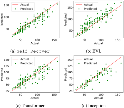
Table 1 compares the forecasting performance of the various methods in terms of their RMSE and correlation. The results show that the proposed Self-Recover framework outperformed all the baselines on both Hurricane and Climate datasets. To further validate the significance of the results, we conducted a t-test and computed the p-values of the difference in RMSE and correlation between Self-Recover against the best baseline method for the 10 runs of each dataset. For Hurricane data, we obtain p = 0.00025 for RMSE and p = 0.00067 for correlation, while for Climate data, p = 0.02704 for RMSE and p = 0.00379 for correlation. These suggest that the improvements are statistically significant. To verify its effectiveness in terms of modeling extreme values, Figure 4 shows the scatter plots of the actual versus predicted block maxima values for Self-Recover, EVL, Transformer, and Inception on the Hurricane intensity data. The plots indicate that Self-Recover can accurately estimate the block maxima values of hurricane intensity. In contrast, the block maxima predictions generated by other competing baselines have larger biases.
| Imputation Methods | Hurricane | Climate | ||
|---|---|---|---|---|
| RMSE | Correlation | RMSE | Correlation | |
| Randomized | 5.21 ± 0.31 | 0.70 ± 0.05 | 2.81 ± 0.28 | 0.73 ± 0.05 |
| Self-supervised | 4.51 ± 0.36 | 0.78 ± 0.04 | 2.26 ± 0.24 | 0.81 ± 0.03 |
Finally, Table 2 compares the accuracy of each method in terms of classifying extremely high hurricane intensity and temperature events. Observe that Self-Recover outperforms all other baselines in terms of accuracy and F1 score.
Effect of Self-supervised Missing Value Imputation. Table 3 compares the missing value imputation performance of Self-Recover against random imputation with Gaussian distribution. The results show that our self-supervised imputation approach significantly outperformed random imputation in terms of RMSE and correlation on all datasets.
Effect of Residual Learning. Table 4 compares the performance of Self-Recover when using simple concatenation to combine its learned representations against the residual learning approach. While their accuracies are quite similar, the training runtime for the simple concatenation approach is significantly higher due to its slower convergence.
| Methods | Hurricane | Climate | ||
|---|---|---|---|---|
| RMSE | Runtime (s) | RMSE | Runtime (s) | |
| Concatenation | 14.95 ± 0.23 | 1503.4 | 2.86 ± 0.24 | 1012.7 |
| Residual | 14.88 ± 0.22 | 1215.9 | 2.79 ± 0.26 | 891.6 |
4.3 Ablation Studies
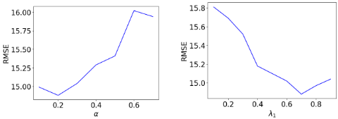
We examine the effects of varying two hyperparameters of our algorithm, α, and λ1. The hyperparameter α determines the residual weight of the model-based representation when combined with the historical representation. As shown in Figure 5 (left), the RMSE generally increases with increasing value of α. For both data sets, a smaller value of α results in higher performance, which validates our strategy for incorporating the model-based representation as a "residual" term to enhance the representation of historical observations.
The trade-off between minimizing point prediction (RMSE loss) and preserving the GEV distribution (GEV loss) of Self-Recover is determined by the hyperparameter λ1 in Equation 14. A larger λ1 places greater emphasis on GEV loss, which focuses more on extreme values. This can be seen from the results shown in Figure 5 (right), where the RMSE of the block maxima prediction decreases when λ1 increases. This suggests that the combined loss is useful rather than using only the RMSE loss, thus validating the need to incorporate GEV distribution into the Self-Recover framework.
5 Conclusion
This paper introduces Self-Recover, a novel deep learning framework for predicting the block maxima of time series by handling disparate temporal coverage of predictors. A combination of contrastive and generative self-supervised learning schemes followed by a DAE is proposed to impute the structured and random missing values present in modelbased forecasts. To learn and merge the representations from historical and model-based forecasts, we provide a residual technique and show that it is more efficient than the straightforward concatenation method. Experimental results on realworld data demonstrate the superiority of Self-Recover compared to other state-of-the-art methods.
Acknowledgments
This research is supported by the U.S. National Science Foundation under grant IIS-2006633. Any use of trade, firm, or product names is for descriptive purposes only and does not imply endorsement by the U.S. Government.
@inproceedings{ijcai2023p414,
  title     = {Self-Recover: Forecasting Block Maxima in Time Series from Predictors with Disparate Temporal Coverage Using Self-Supervised Learning},
  author    = {Galib, Asadullah Hill and McDonald, Andrew and Tan, Pang-Ning and Luo, Lifeng},
  booktitle = {Proceedings of the Thirty-Second International Joint Conference on
               Artificial Intelligence, {IJCAI-23}},
  publisher = {International Joint Conferences on Artificial Intelligence Organization},
  editor    = {Edith Elkind},
  pages     = {3723--3731},
  year      = {2023},
  month     = {8},
  note      = {Main Track},
  doi       = {10.24963/ijcai.2023/414},
  url       = {https://doi.org/10.24963/ijcai.2023/414},
}
TY - CPAPER TI - Self-Recover: Forecasting Block Maxima in Time Series from Predictors with Disparate Temporal Coverage Using Self-Supervised Learning AU - Galib, Asadullah Hill AU - McDonald, Andrew AU - Tan, Pang-Ning AU - Luo, Lifeng T2 - Proceedings of the Thirty-Second International Joint Conference on Artificial Intelligence, IJCAI-23 PB - International Joint Conferences on Artificial Intelligence Organization PY - 2023 SP - 3723 EP - 3731 DO - 10.24963/ijcai.2023/414 UR - https://doi.org/10.24963/ijcai.2023/414 ER -Copied
Machine-readable versions of this paper, for tools and AI agents:





