
BayCon: Model-agnostic Bayesian Counterfactual Generator
Proceedings of the Thirty-First International Joint Conference on Artificial Intelligence. Main Track. Pages 740-746.
https://doi.org/10.24963/ijcai.2022/104
Keywords
- Machine Learning: Hyperparameter Optimization
- AI Ethics, Trust, Fairness: Trustworthy AI
- Constraint Satisfaction and Optimization: Applications
- AI Ethics, Trust, Fairness: Explainability and Interpretability
Abstract
Generating counterfactuals to discover hypothetical predictive scenarios is the de facto standard for explaining machine learning models and their predictions. However, building a counterfactual explainer that is time-efficient, scalable, and model-agnostic, in addition to being compatible with continuous and categorical attributes, remains an open challenge. To complicate matters even more, ensuring that the contrastive instances are optimised for feature sparsity, remain close to the explained instance, and are not drawn from outside of the data manifold, is far from trivial. To address this gap we propose BayCon: a novel counterfactual generator based on probabilistic feature sampling and Bayesian optimisation. Such an approach can combine multiple objectives by employing a surrogate model to guide the counterfactual search. We demonstrate the advantages of our method through a collection of experiments based on six real-life datasets representing three regression tasks and three classification tasks.
- [Breunig et al., 2020] Markus M. Breunig, Hans-Peter Kriegel, Raymond T. Ng, and Jörg Sander. LOF: Identi- fying density-based local outliers. In Proceedings of the 2000 ACM SIGMOD international conference on man- agement of data, pp. 93-104, 2000.
- [Brochu et al., 2010] Eric Brochu, Vlad M. Cora, and Nando De Freitas. A tutorial on Bayesian optimisation of expen- sive cost functions, with application to active user model- ing and hierarchical reinforcement learning. arXiv pre- print arXiv:1012.2599, 2010.
- [Byrne, 2005] Ruth M. J. Byrne. The rational imagination: How people create alternatives to reality. MIT Press, Cambridge, Massachusetts, 2005.
- [Byrne, 2019] Ruth M. J. Byrne. Counterfactuals in explain- able artificial intelligence (XAI): Evidence from human reasoning. In IJCAI, pp. 6276-6282. 2019. IJCAI
- [Cui et al., 2015] Zhicheng Cui, Wenlin Chen, Yujie He, and Yixin Chen. Optimal action extraction for random forests and boosted trees. In Proceedings of the 21 st ACM SIGKDD International Conference on Knowledge Dis- covery and Data Mining, pp. 179-188, 2015.
- [Dandl et al., 2020] Susanne Dandl, Christoph Molnar, Mar- tin Binder, and Bernd Bischl. Multi-objective counterfac- tual explanations. In International Conference on Parallel Problem Solving from Nature, pp. 448-469. Springer, Cham, 2020.
- [Dhurandharetal et al., 2018] Amit Dhurandhar, Pin Yu Chen, Ronny Luss, Chun-Chen Tu, Paishun Ting, Karthikeyan Shanmugam, and Payel Das. Explanations based on the missing: Towards contrastive explanations with pertinent. In NIPS, pp. 590-601, 2018.
- [Gjoreski et al., 2020] Martin Gjoreski, Vladimir Kuz- manovski, and Marko Bohanec. Generating alternatives for DEX models using Bayesian optimization. Proceed- ings of the 23 rd International Multiconference Information Society, 2020.
- [Gjoreski et al., 2022] Martin Gjoreski, Vladimir Kuz- manovski, and Marko Bohanec. BAG-DSM: A Method ` for Generating Alternatives for Hierarchical Multi-Attrib- ute Decision Models using Bayesian Optimization. Algo- rithms, 15, 1972022, 2022.
- [Goodman and Flaxman, 2017] Bryce Goodman, and Seth Flaxman. European Union regulations on algorithmic de- cision-making and a "right to explanation", AI Magazine 38 (3) 50-57, 2017.
- [Hoffman et al., 2018] Robert Hoffman, Tim Miller, Shane T. Mueller, Gary Klein, and William J. Clancey. Explain- ing explanation, part 4: A deep dive on deep nets. IEEE Intelligent Systems 33, no. 3:87-95, 2018.
- [Hutter et al., 2011] Frank Hutter, Holger H. Hoos, and Kevin Leyton-Brown. Sequential model-based optimisation for general algorithm configuration. In International Confer- ence on Learning and Intelligent Optimisation, Springer, 2011.
- [Keane et al., 2021] Mark T. Keane, Eoin M. Kenny, Eoin Delaney, and Barry Smyth. If only we had better counter- factual explanations: Five key deficits to rectify in the evaluation of counterfactual XAI techniques. In IJCAI, pp. 4466-4474. 2021. IJCAI
- [Kentaro et al., 2020] Kanamori Kentaro, Takuya Takagi, Ken Kobayashi, and Hiroki Arimura. DACE: Distribu- tion-aware counterfactual explanation by mixed-integer linear optimization. In IJCAI, pp. 2855-2862. 2020. IJCAI
- [Lash et al., 2017] Michael T. Lash, Qihang Lin, W. Nick Street, Jennifer G. Robinson, and Jeffrey W. Ohlmann. Generalised inverse classification. In Proceedings of the SIAM International Conference on Data Mining, pp. 162- 170, 2017.
- [Laugel et al., 2019] Thibault Laugel, Marie-Jeanne Lesot, Christophe Marsala, Xavier Renard and Marcin Detyniecki. The dangers of post-hoc interpretability. In IJCAI-19, pp. 2801-2807, 2019.
- [Lizotte, 2008] Daniel James Lizotte. Practical Bayesian op- timization. PhD Thesis, University of Alberta, Depart- ment of Computing Science, 2008.
- [Močkus, 1974] Jonas Močkus, On Bayesian methods for seeking the extremum. IFIP Technical Conference on Op- timization Techniques (pp. 400-404). Springer, 1974.
- [Moore et al., 2019] Jonathan Moore, Nils Hammerla, and Chris Watkins. Explaining deep learning models with constrained adversarial examples. In Proceedings of the 16th Pacific Rim International Conference on Artificial Intelligence, pp. 43-56, 2019.
- [Pedregosa et al., 2011] Fabian Pedregosa, Gaël Varoquaux, Alexandre Gramfort, Vincent Michel, Bertrand Thirion, Olivier Grisel, Mathieu Blondel, et al. scikit-learn: Ma- chine learning in Python. The Journal of Machine Learn- ing research. 12:2825-30, 2011.
- [Poyiadzi et al., 2020] Rafael Poyiadzi, Kacper Sokol, Raul Santos-Rodriguez, Tijl De Bie, Peter Flach. FACE: Fea- sible and actionable counterfactual explanations. In Pro- ceedings of the AAAI/ACM Conference on AI, Ethics, and Society pp. 344-350, 2020.
- [Rasmussen et al., 2006] Carl Edward Rasmussen, and Chris- topher K. I. Williams. Gaussian Processes for Machine Learning. Cambridge: The MIT Press, 2006.
- [Rudin, 2019] Cynthia Rudin. Stop explaining black box ma- chine learning models for high stakes decisions and use interpretable models instead. Nature Machine Intelligence 1, no. 5:206-215, 2019.
- [Russell, 2019] Chris Russell. Efficient search for diverse co- herent explanations. In Proceedings of the Conference on Fairness, Accountability, and Transparency, 2019.
- [Snoek et al., 2015] Jasper Snoek, Oren Rippel, Kevin Swersky, Ryan Kiros, Nadathur Satish, Narayanan Sundaram, Mostofa Patwary, Mr Prabhat, and Ryan Ad- ams. Scalable Bayesian optimisation using deep neural networks. In International conference on machine learn- ing, pp. 2171-2180. PMLR, 2015.
- [Sokol et al., 2020] Kacper Sokol, Alexander Hepburn, Ra- fael Poyiadzi, Matthew Clifford, Raul Santos-Rodriguez, and Peter Flach. FAT Forensics: A Python toolbox for im- plementing and deploying fairness, accountability and transparency algorithms in predictive systems. Journal of Open Source Software 5, no. 49 (2020): 1904, 2020.
- [Vanschoren et al., 2014] Joaquin Vanschoren, Jan N. Van Rijn, Bernd Bischl, and Luis Torgo. OpenML: Networked science in machine learning. ACM SIGKDD Explorations Newsletter 15, no. 2 (2014): 49-60, 2014.
- [Wachter et al., 2017] Sandra Wachter, Brent Mittelstadt, and Chris Russell. Counterfactual explanations without open- ing the black box: Automated decisions and the GDPR. Harvard journal of law & technology, 31:841-887, 2017.
References were extracted automatically from the PDF and may contain errors.
Full text extracted automatically from the PDF; figures, tables and equations may differ. The PDF is the version of record.
1 Introduction
The "right to explanation" foreshadowed by the General Data Protection Regulation (GDPR) [Goodman and Flaxman, 2017] challenged the Machine Learning (ML) community to build explainability into predictive models and their outputs. This paradigm shift - where predictive performance is no longer the only (and main) objective - gives rise to two distinct viewpoints. One argues that algorithmic black boxes should continue to be optimised for predictive power with explainability needs, possibly, fulfilled through post-hoc methods due to an apparent incompatibility of these two goals, thus forcing one of them to be sacrificed for the other. 2 The second standpoint disputes this trade-off as purely anecdotal and persuasively argues for building inherently transparent models, especially for high-stakes decisions [Rudin, 2019].
1 * Equal contribution.
`
Counterfactuals are an explainability approach uniquely positioned in this space as they can be generated post-hoc but remain truthful with respect to the underlying black box (i.e., exhibit full fidelity). They enable ML users to understand what the output of a predictive model would have been had the instance in question changed in a particular way. This type of counterfactual analysis helps the explainees to simulate certain aspects of the ML model, thus improving its interpretability [Hoffman et al., 2018]. Notably, evidence from psychology and cognitive sciences suggests that people use counterfactual reasoning daily to analyse what could have happened had they acted differently [Byrne, 2005].
However, the number of counterfactuals that can be generated to explain any event (a selected datapoint) may be overwhelming [Byrne, 2019]. In addition to a large counterfactual search space, methods that are currently available tend to work for either classification or regression tasks, be restricted to a specific model family (e.g., differentiable predictors), struggle with large datasets (both in the number of instances and features), be computationally inefficient, or output outof-distribution counterfactuals. Building on our previous work in the domain of decision support systems [Gjoreski et al., 2020; Gjoreski et al., 2022], we address the existing challenges with BayCon: a novel model-agnostic Bayesian counterfactual generator. To the best of our knowledge, it is the first counterfactual explainer based on Bayesian optimisation, making it fast to produce a sizeable number of highquality contrastive instances. Our approach is model-agnostic and compatible with regression and classification tasks. It outperforms other state-of-the-art counterfactual generation methods on six real-life datasets, which illustrates its effectiveness. Our evaluation uses three regression and three classification datasets with between 8 to 125 categorical and numerical attributes, demonstrating BayCon's speed and versatility. Existing methods for generating counterfactual explanations focus predominantly on differentiable models applied to continuous features [Wachter et al., 2017; Dhurandhar et al., 2018; Moore et al., 2019, Lash et al., 2017]. This creates a blind spot for non-differentiable models trained on datasets with mixed feature types, which are relatively ubiquitous [Rudin, 2019]. To address this gap, several authors proposed (Mixed) Integer Programming approaches [Cui et al., 2015; Russell, 2019; Kentaro et al., 2020]. Another counterfactual generation method, which is somewhat similar to BayCon, is Multi-Objective Counterfactual Explanations (MOC) [Dandl et al., 2020]. MOC is model-agnostic, compatible with regression and classification tasks, and capable of processing numerical and categorical features. Given that both MOC and BayCon attempt to address the same set of counterfactual generation shortcomings, albeit with different approaches, we directly compare them in a set of experiments using six diverse evaluation metrics (see Tables 2 and 3). Additionally, we show how BayCon complies with recent guidelines for designing counterfactual generation methods, thus making it the preferred approach [Keane et al., 2021].
2 https://www.wired.com/story/googles-ai-guru-computersthink-more-like-brains/
2. Preliminaries
Given an instance selected to be explained for a pre-trained ML model, BayCon generates similar instances that lead to the desired prediction, i.e., counterfactuals. A naïve approach is to generate all the possible feature-value combinations or to iteratively generate random instances, discarding the ones with unchanged prediction. However, for datasets with a considerable number of features this search space can be overwhelmingly large, rendering the naïve approaches impractical. A more appropriate strategy could use an informed search based on the record of previously generated and evaluated counterfactuals. These datapoints can be used to map the search space and the behaviour of the ML model. Based on this approximation, promising counterfactuals can be generated more efficiently. Bayesian optimisation can be a vehicle to realise such an informed search stochastically.
2.1. Counterfactual Explanations Desiderata
The BayCon optimisation pipeline is designed to produce contrastive explanations of the highest quality, both with respect to their technical and social properties. To this end, our method adheres to the latest guidelines prescribing how to generate desirable counterfactuals [Keane et al., 2021].
What's Plausible? BayCon optimises for plausibility by minimising the distance to the explained instance in addition to automatically extracting feature constraints from the underlying training dataset. Moreover, our method allows the user to specify immutable features such as age, and indicate attribute values that are invalid, e.g., fractional number of rooms in a house. All these restrictions are used to guide quasi-random feature sampling (explained in Section 3.4).
The Shape of Sparsity. Counterfactuals should strive to tweak the smallest possible number of features to make the explanations parsimonious, hence appealing to humans [Keane et al., 2021]. However, the desired level of sparsity may depend on the user and the dataset, therefore we incorporate the number of altered feature values into the optimisation function used by BayCon. Additionally, the user can specify the maximum number of altered features.
Covering Coverage. Counterfactuals should be feasible and actionable [Poyiadzi et al., 2020]. In particular, out-of-
`
distribution counterfactuals - which can amount to 36% of all the generated explanations for some methods - should be avoided [Laugel et al., 2019]. BayCon uses Local Outlier Factor (LOF) to prevent such counterfactuals from being presented to the explainee.
Comparative Testing. BayCon is compared to state-of-theart counterfactual explainers on six publicly available datasets using well-defined evaluation metrics.
2.2. Optimisation Objective
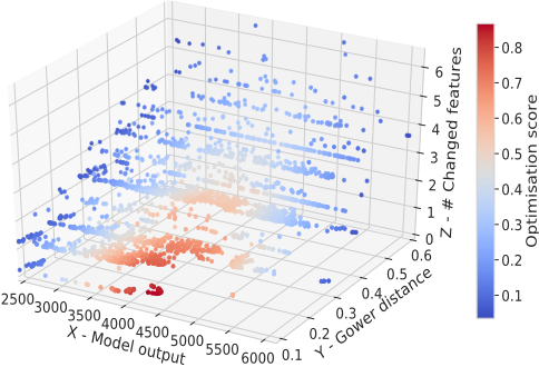
To assess the quality of generated counterfactual explanations, we designed a suitable objective function. It captures: (1) the distance in the feature space, (2) the distance in the output space, and (3) the number of altered features, all scaled to the [0, 1] range. Figure 1 shows example optimisation scores for the Bike dataset (cf. Table 1). Each point in the plot is a candidate counterfactual. The x-axis represents the output of the ML model for which we are generating counterfactuals; the y-axis shows the Gower distance between each counterfactual and the explained instance; the z-axis captures the number of changed features; and the marker colour indicates the optimisation score calculated with Equation 1 (higher is better). In this example, the explained instance is predicted as 3141 (rented bikes), and the desired output range (provided by the explainee) is set to [4500, 5000]. The figure shows that: (i) the optimisation scores for counterfactuals whose predictions (y-axis) are outside of the user-specified range are close to 0 and increase as the model's output approaches the desired range; (ii) the optimisation scores decrease as the Gower distance increases; and (iii) the optimisation scores are higher for counterfactuals that require a lower number of features to be changed.
Similarity in the feature space (𝑆!). Gower distance is a distance metric used for mixed feature spaces. For categorical attributes, it checks whether the two features have an identical value - the distance component is 0 if the features are the same and 1 otherwise. For numerical features, it calculates the absolute value of the difference between the attributes, divided by the numerical range of the feature. All of these individual components are then added up and divided by the number of attributes, which places the distance in the [0, 1] range. Next, we integrate this metric - the Gower distance between the explained instance 𝑥̅ and a counterfactual candidate 𝑐 $ - into our optimisation function (𝑆! in Equation 2) by subtracting it from 1:
Similarity in the output space (𝑆"). For classification tasks, 𝑆" is 1 if the ML model predicts the candidate counterfactual as requested by the user, and 0 otherwise. For regression problems, we define 𝑆" as:
In Equation 3, 𝑦! is the output of the ML model for the explained instance; 𝑦) is the output of the ML model for the candidate counterfactual; and [𝑦*+, , 𝑦*/0 ] is the target output range specified by the user. If 𝑦) is in the desired range, 𝑆" = 1 (the maximum value). Otherwise, 𝑆𝑦 captures the closeness of 𝑦) to the borders (calculated via 𝑑) of the desired range. 𝑆𝑦 is designed to be within the [0, 1] interval.
Proportion of tweaked features (𝑆#). This objective counts the number of features in the candidate counterfactual that are different when compared to the explained instance. This score is also in the [0, 1] range - see Equation 5.
For comparison, MOC formalises counterfactual search as a multi-objective optimisation problem solved with Nondominated Sorting Genetic Algorithm II (NSGA-II). The objectives used by MOC are: (i) prediction closeness to the desired goal, (ii) closeness to the initial instance in the feature space, (iii) number of changed features, and (iv) plausibility of counterfactual candidates based on the probability distribution over the feature values. BayCon mirrors objectives (i), (ii) and (iii) with the aforementioned scores: 𝑆", 𝑆!, and 𝑆# respectively. Objective (iv) is addressed implicitly by the LOF filtering.
`
3 Methodology
Bayesian optimisation allows utilising prior beliefs about a problem to help navigate the sampling. This is achieved by following a simplified version of the Bayes' theorem: the posterior probability of a function F given data D (or evidence) is proportional to the likelihood of D (given F) and the prior probability of F:
In our case, 𝐷 consists of n observed counterfactuals and their black-box prediction: D = {(𝑐:, EEE 𝐹(𝑐;, EEE 𝑥̅ )), … , (𝑐8, EEEE 𝐹(𝑐8, EEEE 𝑥̅ ))}.
3.1 Surrogate Model
To estimate the posterior of our objective function (Equation 6), we employ a surrogate model. It is an ML model typically learnt with regression algorithms based on a Gaussian Process (GP) because such a model provides access to the full probability distribution [Snoek et al., 2015, Rasmussen et al., 2006]. By exploiting the mean and the standard deviation of the output distribution, one can balance the exploitation (higher mean) and exploration (higher standard deviation) trade-off. Since GPs are computationally expensive - 𝑂(𝑛< ) complexity - ensemble regression models such as Random Forests can be used instead [Hutter et al., 2011]. In such a case, the mean and variance are calculated based on the predictions of all the individual models within the ensemble. In our case, the input of the surrogate model is defined as:
In this equation ∆𝑘7 represents the distance between 𝑐̅ and 𝑥 $ for feature 𝑖; 𝑐𝑜𝑢𝑛𝑡(∆𝑘) is the number of features changed in 𝑐̅ as compared to 𝑥 $; and the last input is the Gower distance between 𝑐 $ and 𝑥̅ . Therefore, for any given input the surrogate model outputs an estimation of our optimisation score.
3.3 Acquisition Function
The mean µ(𝑆) $) and variance 𝜎(𝑆) $) calculated on the output of the surrogate model are used as input to an acquisition function, which is responsible for selecting the most promising counterfactuals. This function optimises the conditional probability of the feature space to identify regions with promising counterfactuals. BayCon uses Expected Improvement as its acquisition function [Močkus, 1974]. In our experiments, the constant that controls the trade-off between global search and local optimisation (i.e., exploration/exploitation) is set to ξ = 0.01 [Lizotte et al. 2008, Brochu et al., 2010]. Intuitively, this acquisition function checks the improvement that each candidate counterfactual brings with respect to the maximum known value 𝑆=, i.e., µ(𝑆) $) -𝑆=, and scales this improvement with respect to the uncertainty given by 𝜎(𝑆) $). If two counterfactuals have a similar mean value, the one with higher uncertainty is preferred by the acquisition function.
3.4 Generating Candidate Counterfactuals
Initial Neighbourhood Generation. Given the assumption that good counterfactuals should be close to the explained instance, our search is focused on its neighbourhood. To generate this space, for each feature we sample values at random with replacements from a truncated (based on the feature ranges) normal distribution centred around the initial instance. Categorical attributes are sampled uniformly over the set of possible values.
Exploring Best Counterfactual Neighbourhoods. Since good counterfactuals should come from dense regions, we explore neighbourhoods of explanations with best scores. We reuse the generation procedure applied to the initial instance, this time centred around the best counterfactuals.
Random Feature Sampling. To enable a higher degree of exploration, we sample values of numerical features uniformly at random from within their ranges. Categorical attributes are sampled uniformly over the set of possible values.
Rounding. To avoid indistinguishable counterfactuals that only differ beyond an n th decimal place for numerical features, we perform k-bins discretisation with equal-width bins. We used k = 100 for our experiments, which provides the minimum difference of 1% relative to the attribute range.
Selecting Features to Be Tweaked. To increase sparsity, i.e., change the fewest possible features per counterfactual, we randomly select attributes to update based on a skewed distribution where the probability of changing n features is double that of changing n+1. Only the selected features are then updated using the procedure described in the previous steps (neighbourhood generation or random sampling).
Filtering. BayCon is an iterative algorithm. At each step, we prune candidate counterfactuals whose score is below the current best. Also, prior to outputting the explanations, we remove out-of-distribution counterfactuals with LOF, which measures the local density deviation of each explanation with respect to its neighbourhood determined by the training dataset. Explanations that have a substantially lower density than their neighbours are therefore removed. For this purpose, we use scikit-learn's LOF implementation with default parameters [Breunig et al., 2000]. Algorithm 1 captures our implementation of BayCon in more detail. The maximum number of iterations was set to 100.
4 Experiments
We compare BayCon against other counterfactual generation methods on six real-life datasets. Our method is implemented in Python 3.6 and relies heavily on scikit-learn [Pedregosa et al., 2011]. All the experiments were run on a 3.70GHz Intel Core i9 CPU with 128GB of RAM. We imposed a 15-minute runtime limit for each execution. BayCon implementation and the experimentation code, including processed datasets and analysis of the results, are freely available on GitHub 3 .
`
3 https://github.com/piotromashov/baycon
Algorithm 1 BayCon.
Input: black-box-model f, instance to be explained x*, desired prediction p, training data 𝑋?. Output: counterfactuals CFs.
- 1: X = generate neighbourhood (x*)
- 2: y = f (X) # predict neighbourhood
- 3: 𝑆@ = objective function (X, y, p) # calculate scores
- 4: 𝑋A, 𝑦A = update known instances (X, y)
- 5: g = RandomForest (𝑋A, 𝑆@) # train surrogate model
6:
- 7: while continue search do
- 8: CF = select counterfactuals (𝑋A, 𝑦A)
- 9: 𝐶𝐹=, 𝑆= = select best (CF, 𝑆@)
- 10: X = generate neighbourhood (𝐶𝐹=)
- 11: 𝑋B = update promising instances (X)
- 12: X += random generation (𝑆=)
- 13: µ, 𝜎 = g (X)
- 14: 𝑋C = acquisition function rank (X, µ, 𝜎)
- 15: y = f (𝑋C) # get black-box predictions
- 16: 𝑆@ += objective function (𝑋C, y, p)
- 17: 𝑋A = update known instances (𝑋C, y)
- 18: g.retrain (𝑋A, 𝑆@) # update surrogate model
- 19: end while
20:
- 21: y = f (𝑋B) # get black-box predictions
- 22: CFs += update with counterfactuals from (𝑋B, y)
- 23: CFs = LOF filter (CFs, 𝑋?)
- 24: return CFs
4.1 Experimental Setting
We compare our proposed method to a brute-force exhaustive counterfactual search implemented in FAT Forensics [Sokol et al. 2020] and MOC based on its official implementation. FAT Forensics only yielded explanations for the Diabetes dataset given the imposed 15-minute time limit, hence it is not featured in our comparison. MOC, on the other hand, generated explanations for all the datasets but the House Sales (likely due to the size of its training set) as it is a stateof-the-art method.
For the comparison we used three classification (Cls) and three regression (Reg) datasets (see Table 1 and Appendix A for more information). All the datasets are available online; the Bike dataset can be downloaded from the UCI repository and the other datasets are available through the OpenML repository [Vanschoren et al. 2014].
For each classification dataset we selected 10 random instances to be explained, generating their counterfactual explanations 3 times to account for randomness (i.e., 30 runs per dataset). For each regression dataset, we selected 3 initial instances, one for each percentile of the output variable: the median as well as the 25 th (𝑦;> in Equation 7) and the 75 th percentiles. Next, we generated explanations for 4 desired target ranges - to increase, to decrease, to be in an interval above (𝑦! +𝑎, 𝑦! +𝑏) and to be in an interval below (𝑦! - 𝑏, 𝑦! -𝑎) the prediction of the explained instance, with a and b defined in Equation 8. Each experiment was repeated 3 times (i.e., 36 runs per dataset).
| Dataset | Features (Num/Cat) | Type | Samples |
|---|---|---|---|
| Diabetes | 8/0 | Cls | 768 |
| Kc2 | 22/0 | Cls | 522 |
| Biodeg | 41/0 | Cls | 1055 |
| Bike | 7/3 | Reg | 730 |
| House Sales | 19/2 | Reg | 21613 |
| Tecator | 125/0 | Reg | 240 |
We explained predictions of two black-box models: a Random Forest (RF) and a Support Vector Machine (SVM). The models were trained with all the data, excluding the explained instances. Since SVMs can be sensitive to feature scaling and model parameterisation, we applied min-max normalisation to the input features and tuned the model parameters using 3fold cross-validation on the training data.
4.2 Experimental Results
Table 2 compares BayCon and MOC with respect to the total compute time, the time to first solution and the number of generated counterfactuals (all times given in seconds). The time to first solution for MOC was calculated as the total time divided by the number of generated explanations. While such
| Method | Total t | t to 1 st CF | #CFs | |
|---|---|---|---|---|
| Diabetes | BC | 3.5(1) | 0.1(0) | 398(173) |
| MOC | 80.7(40) | 1.6(1) | 58(28) | |
| Kc2 | BC | 9.0(5) | 0.4(1) | 2529(1437) |
| MOC | 192.1(133) | 8.5(21) | 45(19) | |
| Biodeg | BC | 13.2(9) | 0.3(0) | 1138(755) |
| Bike | MOC BC | 302.7(167) 4.7(2) | 4.5(8) 0.0(0) | 100(49) 1446(493) |
| MOC | 47.6(27) | 1.1(2) | 78(56) | |
| H. Sales | BC MOC | 26.2(4) / | 0.2(0) / | 1723(674) / |
| Tecator | BC | 83.3(34) | 0.1(1) | 42949(20154) |
| MOC | 429.1(98) | 155.5(52) | 3(1) | |
| Average | BC | 23.3(9.2) | .18(.33) | 8363(3947) |
| MOC | 210.4(93) | 3.16(17) | 47(25) |
`
a strategy gives MOC an advantage, BayCon outperformed it across the board. Additionally, the House Sales dataset caused MOC to timeout, which is likely due to the size of the training dataset.
Table 3 outlines the experimental comparison between BayCon and MOC using the three evaluation scores - 𝑆", 𝑆#, 𝑆! - proposed in Section 2. It presents the mean and standard deviation for each score and the accompanying result of the Mann-Whitney U rank test. The sample size, which depends on the number of counterfactuals generated in each experimental run, is also shown - a sample size of 833 indicates that for this experiment we compared the scores of 833 explanations generated by MOC with the same number of explanations generated by BayCon. Since the methods could generate a different number of explanations, we only took the top n counterfactuals (ranked by the evaluation score) with n determined by the smallest number of explanations generated for a given experimental setup across the two methods. Bolded p-values highlight the experiments in which BayCon outperformed MOC with statistical significance (p<0.05). This happened in most of the experiments, except for the Bike and the Tecator datasets predicted with an SVM, but only when measured by the 𝑆" score. In these specific experiments, MOC found better counterfactuals in the output space (𝑆"), however BayCon found better counterfactuals in the feature space (𝑆# and 𝑆!). Notably, BayCon offered counterfactuals with a smaller number of changed features and smaller Gower distance across all experiments.
5 Conclusions and Future Work
Our experiments demonstrated that, compared to state-ofthe-art methods, BayCon is more time-efficient and generates larger and more diverse sets of counterfactuals (see Table 2). Furthermore, the explanations output by our algorithm are of better quality: they are placed closer to the explained instance and require fewer feature tweaks, thus making them more similar to it. In future work, we will address the counterfactual multiplicity by exploring various filtering, pruning and selection methods. We will also investigate visualisation techniques to help the users better navigate the output explanations and select them based on (possibly implicit) user preferences. Moreover, we will conduct user studies to analyse the perceived quality and benefit of BayCon's counterfactuals to avoid "neglecting the users" [Keane et al., 2021].
Appendices
A. Datasets
Diabetes: https://www.openml.org/d/37
KC2: https://www.openml.org/d/1063
Biodeg: https://openml.org/d/1494
Bike: http://archive.ics.uci.edu/ml/datasets/Bike+Sharing+Dataset
House: https://www.openml.org/d/42731
Tecator: https://www.openml.org/d/505
| Bike Kc2 833) SVM M BC .69 .72 .49 .23 p<0.001 p<0.001 Diabetes 1,002) SVM M BC .89 1.0 .10 0.0 p<0.001 p>.05 Biodeg 1,437) SVM M BC 1.0 1.0 .007 1.0 p<0.001 p>.05 |
- [Byrne, 2019] Ruth M. J. Byrne. Counterfactuals in explainable artificial intelligence (XAI): Evidence from human reasoning. In IJCAI, pp. 6276-6282. 2019.
[Cui et al., 2015] Zhicheng Cui, Wenlin Chen, Yujie He, and Yixin Chen. Optimal action extraction for random forests and boosted trees. In Proceedings of the 21 st ACM SIGKDD International Conference on Knowledge Discovery and Data Mining, pp. 179-188, 2015.
- [Dandl et al., 2020] Susanne Dandl, Christoph Molnar, Martin Binder, and Bernd Bischl. Multi-objective counterfactual explanations. In International Conference on Parallel Problem Solving from Nature, pp. 448-469. Springer, Cham, 2020.
- [Dhurandharetal et al., 2018] Amit Dhurandhar, Pin Yu Chen, Ronny Luss, Chun-Chen Tu, Paishun Ting, Karthikeyan Shanmugam, and Payel Das. Explanations based on the missing: Towards contrastive explanations with pertinent. In NIPS, pp. 590-601, 2018.
- [Gjoreski et al., 2020] Martin Gjoreski, Vladimir Kuzmanovski, and Marko Bohanec. Generating alternatives for DEX models using Bayesian optimization. Proceedings of the 23 rd International Multiconference Information Society, 2020.
- [Gjoreski et al., 2022] Martin Gjoreski, Vladimir Kuzmanovski, and Marko Bohanec. BAG-DSM: A Method
Acknowledgements
The work at Università della Svizzera italiana was supported by the Swiss National Science Foundation, project 200021_182109 (BASE: Behavioral Analytics for Smart Environments). Kacper Sokol was supported by the ARC Centre of Excellence for Automated Decision-Making and Society, funded by the Australian Government through the Australian Research Council (project number CE200100005).
@inproceedings{ijcai2022p104,
  title     = {BayCon: Model-agnostic Bayesian Counterfactual Generator},
  author    = {Romashov, Piotr and Gjoreski, Martin and Sokol, Kacper and Martínez, María Vanina and Langheinrich, Marc},
  booktitle = {Proceedings of the Thirty-First International Joint Conference on
               Artificial Intelligence, {IJCAI-22}},
  publisher = {International Joint Conferences on Artificial Intelligence Organization},
  editor    = {Luc De Raedt},
  pages     = {740--746},
  year      = {2022},
  month     = {7},
  note      = {Main Track},
  doi       = {10.24963/ijcai.2022/104},
  url       = {https://doi.org/10.24963/ijcai.2022/104},
}
TY - CPAPER TI - BayCon: Model-agnostic Bayesian Counterfactual Generator AU - Romashov, Piotr AU - Gjoreski, Martin AU - Sokol, Kacper AU - Martínez, María Vanina AU - Langheinrich, Marc T2 - Proceedings of the Thirty-First International Joint Conference on Artificial Intelligence, IJCAI-22 PB - International Joint Conferences on Artificial Intelligence Organization PY - 2022 SP - 740 EP - 746 DO - 10.24963/ijcai.2022/104 UR - https://doi.org/10.24963/ijcai.2022/104 ER -Copied
Machine-readable versions of this paper, for tools and AI agents:





