
Hierarchical Graph Traversal for Aggregate k Nearest Neighbors Search in Road Networks (Extended Abstract)
Proceedings of the Thirtieth International Joint Conference on Artificial Intelligence. Sister Conferences Best Papers. Pages 4730-4734.
https://doi.org/10.24963/ijcai.2021/640
© 2021 International Joint Conferences on Artificial Intelligence
Keywords
- Multidisciplinary Topics and Applications: Transportation
- Data Mining: Big Data, Large-Scale Systems
- Heuristic Search and Game Playing: Heuristic Search
Abstract
A k nearest neighbors (kNN) query finds k closest points-of-interest (POIs) from an agent's location. In this paper, we study a natural extension of the kNN query for multiple agents, namely, the Aggregate k Nearest Neighbors (AkNN) query. An AkNN query retrieves k POIs with the smallest aggregate distances where the aggregate distance of a POI is obtained by aggregating its distances from the multiple agents (e.g., sum of its distances from each agent). We propose a novel data structure COLT (Compacted Object-Landmark Tree) which enables efficient hierarchical graph traversal and utilize it to efficiently answer AkNN queries. Our experiments on real-world and synthetic data sets show that our techniques outperform existing approaches by more than an order of magnitude in almost all settings.
- [Abeywickrama and Cheema, 2017] Tenindra Abey- wickrama and Muhammad Aamir Cheema. Efficient Landmark-Based Candidate Generation for kNN Queries on Road Networks. In DASFAA, pages 425-440, 2017.
- [Abeywickrama et al., 2016] Tenindra Abeywickrama, Muhammad Aamir Cheema, and David Taniar. k-nearest neighbors on road networks: A journey in experimentation and in-memory implementation. PVLDB, 9(6):492-503, 2016.
- [Abeywickrama et al., 2020] Tenindra Abeywickrama, Muhammad Aamir Cheema, and Sabine Storandt. Hier- archical graph traversal for aggregate k nearest neighbors search in road networks. In ICAPS, pages 2-10, 2020.
- [Akiba et al., 2014] Takuya Akiba, Yoichi Iwata, Ken-ichi Kawarabayashi, and Yuki Kawata. Fast shortest-path dis- tance queries on road networks by pruned highway label- ing. In ALENEX, pages 147-154, 2014.
- [Drews and Luxen, 2013] Florian Drews and Dennis Luxen. Multi-hop ride sharing. In Sixth annual symposium on combinatorial search, 2013.
- [Goldberg and Harrelson, 2005] Andrew V. Goldberg and Chris Harrelson. Computing the shortest path: A* search meets graph theory. In SODA, pages 156-165, 2005.
- [Goldenberg et al., 2011] Meir Goldenberg, Nathan R. Sturtevant, Ariel Felner, and Jonathan Schaeffer. The compressed differential heuristic. In AAAI, 2011.
- [Guttman, 1984] Antonin Guttman. R-trees: A dynamic in- dex structure for spatial searching. In SIGMOD, pages 47- 57, 1984.
- [Stiglic et al., 2015] Mitja Stiglic, Niels Agatz, Martin Savelsbergh, and Mirko Gradisar. The benefits of meeting points in ride-sharing systems. Transportation Research Part B: Methodological, 82:36-53, 2015.
- [Yiu et al., 2005] Man Lung Yiu, Nikos Mamoulis, and Dimitris Papadias. Aggregate nearest neighbor queries in road networks. IEEE Trans. Knowl. Data Eng., 17(6):820- 833, 2005.
- [Zhong et al., 2015] Ruicheng Zhong, Guoliang Li, Kian- Lee Tan, Lizhu Zhou, and Zhiguo Gong. G-tree: An ef- ficient and scalable index for spatial search on road net- works. IEEE Trans. Knowl. Data Eng., 27(8):2175-2189, 2015.
- [Zhu et al., 2010] Liang Zhu, Yinan Jing, Weiwei Sun, Dingding Mao, and Peng Liu. Voronoi-based aggregate nearest neighbor query processing in road networks. In GIS, pages 518-521, 2010.
References were extracted automatically from the PDF and may contain errors.
Full text extracted automatically from the PDF; figures, tables and equations may differ. The PDF is the version of record.
1 Introduction
A kNN query [Zhong et al., 2015] returns k points-of-interest (POIs) closest from an agent's location, e.g., find three closest gas stations to a taxi driver in a given road network. But in many applications (as e.g., ride-sharing [Stiglic et al., 2015; Drews and Luxen, 2013]), it is important to obtain nearby POIs considering the locations of multiple agents. This motivates the consideration of aggregate k nearest neighbors (AkNN) queries [Yiu et al., 2005; Zhu et al., 2010], which are a natural extension of kNN queries that retrieve POIs considering their aggregate distance from all agents. For example, a group of friends might want to decide for a restaurant to meet such that the maximum distance any of them needs to travel is minimized. They can issue an AkNN query to find k restaurants with the smallest aggregate distances where the aggregate function is max.
More formally, given a POI p and a set of agents Q, the aggregate distance of p from the agents is dagg(Q, p) = agg(d(qi, p), ∀qi∈Q) where d(qi, p) denotes the road network distance (e.g., travel time, path length) from an agent qi to p and agg() is an aggregate function. For example, when the aggregate function is sum, dagg(Q, p) = ∑qi∈Q d(qi, p) and when the aggregate function is max, dagg(Q, p) = maxqi∈Q d(qi, p). An AkNN query returns k POIs with the smallest aggregate distances.
∗This is an abridged version of a paper that won the best paper award at ICAPS 2020 [Abeywickrama et al., 2020].
Yiu et al. [Yiu et al., 2005] solve the AkNN query using a hierarchical search on the road network. They utilize an R-tree [Guttman, 1984] which recursively divides POIs into subsets by Minimum Bounding Rectangles (MBRs). During search, a lower-bound aggregate distance for all POIs in a child R-tree node is computed using the Euclidean distances to its MBR. The algorithm visits the most promising R-tree branches to pinpoint result POIs. However, Euclidean distance is only a loose lower-bound especially on metrics like travel time, making the heuristic less efficient. Moreover, the inefficiency is exacerbated for AkNNs as the error will also be aggregated. Landmark Lower-Bounds (LLBs) are better heuristics than Euclidean distance [Goldberg and Harrelson, 2005], however, there does not exist a hierarchical data structure to compute minimum LLBs to groups of POIs in the same way as R-trees using Euclidean distance.
In this paper, we address the above mentioned issues and present two hierarchical indexes, SL-Tree and COLT, which add significantly more landmarks than previous methods resulting in tighter bounds, while keeping the indexes reasonably small. COLT is the first index to support hierarchical traversal of the road network using landmark lower-bounds. We propose a heuristic search algorithm to answer AkNN queries for convexity-preserving aggregate functions such as sum and max. Our experiments demonstrate that our techniques achieve up to three orders of magnitude improvement.
2 Proposed Indexes: SL-Tree and COLT
First, we give some background. A road network is a graph G = (V, E) where V is a vertex set and E is an edge set. Each edge (u, v) ∈ E connects two vertices with weight w(u, v) representing any real positive metric, e.g., length, travel time, toll cost of the edge etc. Network distance d(s, t) is the minimum sum of weights connecting vertices s and t. We consider queries and POIs (also called objects in this paper) to be on graph vertices for simpler exposition.
Landmark lower-bounds, also called differential heuristics [Goldenberg et al., 2011], involve selecting a set L of m "landmark" vertices and then pre-computing distances from each landmark to all vertices in V . (1) gives a lower-bound on network distance dist(q, p) using the triangle inequality. The maximum lower-bound over all m landmarks given by (2) gives a tighter lower-bound and is typically accurate even for small m [Goldberg and Harrelson, 2005].
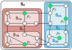
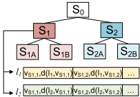
Figure 1: Subgraph Landmark Tree (SL-Tree)
For monotonic aggregate functions, the aggregate of lower-bound distances to object p from each query vertex in Q is a lower-bound LBagg(Q, p) on aggregate distance dagg(Q, p) [Yiu et al., 2005], i.e., LBagg(Q, p) = agg(LB(q1, p), . . . , LB(q|Q|, p)) ≤ dagg(Q, p).
Road network index. We first introduce the SubgraphLandmark Tree (SL-Tree) to index the road network. The SL-Tree is a supporting index that we use to construct our object index efficiently. Each node in the SL-Tree represents a subgraph of the road network with the root being G. G is recursively partitioned into b disjoint subgraphs of equal size, stopping when a subgraph has no more than α vertices. Figure 1a shows such a partitioning for b = 2 and α = 6 with the corresponding SL-Tree shown in Figure 1b. Note that we refer to tree nodes and road network vertices.
For each node nT , we select m of its vertices as local landmarks, e.g., l1 and l2 for m = 2 for S1 in Figure 1a (landmarks for other nodes are omitted for clarity). We then compute distances from each li to every vertex in nT 's subgraph using Dijkstra's search, which are then stored in distance list DLi. Figure 1b shows the distance lists for the landmarks of S1 (those for other nodes are again omitted). Note that subgraphs are stored implicitly by mapping each road network to the SL-Tree leaf node that contains the vertex.
Object index. The SL-Tree can then be used to efficiently construct our object index, the Compacted Object-Landmark Tree (COLT). COLT is a carefully compacted version of the SL-Tree for object set P. Compaction ensures that there are m local landmarks for at most λ objects, to increase the likelihood of finding a tighter lower-bound for more objects. Note that the SL-Tree is shared between construction of all COLT indexes, i.e., for many different object sets.
Given SL-Tree T , COLT index C is constructed by visiting nodes in T in a top-down manner and creating corresponding nodes in C. Let nT be the currently visited node in T (initially the root). A corresponding node nC is created in C for nT . Let λ be the maximum number of objects in a leaf node for COLT. If nT contains more than λ objects, the search expands to its children. Otherwise, the search is pruned at nC, which becomes a leaf-node of COLT. For the new leaf nC, an Object Distance List ODLi is created in nC for each landmark li in nT . These are simply the distance lists of nT , except with only the distances for object vertices from P. Any interior nodes with only one child are merged with the child (keeping the child's more localized landmarks). Figure 2a shows a COLT index for λ = 2 constructed from the SL-Tree in Figure 1b based on the 5 object vertices (green shaded vertices) in Figure 1a. Note that S1A and S1B were removed as construction was pruned at S1 due to its number of objects (ODLs of other nodes are omitted for clarity). While we have chosen λ < α to simplify the example, generally λ ≥ α is required to guarantee no leaf node and therefore no ODL contains more than λ objects. For example, if every vertex in a leaf node is an object there will be α objects in its ODL.
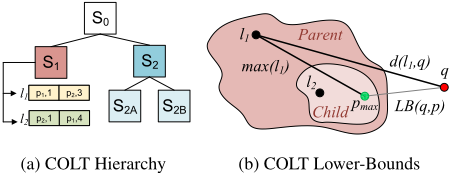
Each object distance list ODLi of leaf node nleaf in C is sorted on distance. In non-leaf nodes nC, we only store the minimumdistanceminnC,li andmaximumdistance maxnC,li to any object in the node from each of its landmarks li. These are computed using distance lists in corresponding SL-Tree nodes. Next, we use this information to compute lower-bounds to nodes and traverse the hierarchy.
2.1 Lower-Bound Heuristic for Graph Traversal
Similar to the lower bound in (1), we can compute a lower bound for all objects contained within a node nC in COLT index C by (3) for one landmark li ∈ nC. (4) gives the best lower-bound over all m landmarks of nC:
Thereby, M - := minnC,li and M + := maxnC,li for nC are already available in COLT. However, for non-root nodes, d(li, q) in (3) is only available if li and q are in the same subgraph. Pre-computing this distance for all V and landmarks is infeasible given the space implications. Alternatively, computing d(li, q) on the fly using another technique is expensive and may be wasteful if the node does not contain results. Interestingly, (3) still holds if we replace the distances with lower-bound LB(li, q) and upper bound UB(li, q), as in
(5). The distance lists of the root or lowest common ancestor SL-Tree node can be used to compute the best LB(li, q) and UB(li, q) by (2) and its upper-bound equivalent (by adding rather than subtracting distances), respectively. Choosing the tightest over all landmarks of nC gives an inexpensive and accurate bound even with a few landmarks:
Landmark choices. We first partition the plane into m equally sized slices around the Euclidean center of the subgraph and then choose one border vertex as a landmark from each slice. If a slice has no borders, we choose the slice vertex furthest from the Euclidean center.
Effective lower-bounds. The accuracy of COLT's inexpensive lower-bounds increases as we delve deeper into the hierarchy. In Figure 2b, let us say we use l1 and its maximum object distance to compute a lower-bound for the child node. At the lower level, we may use the child's landmarks like l2, which are local to the objects and more likely to produce a better lower-bound. This lets us differentiate tree branches and pinpoint the most promising candidates. Next, we utilize this as a decoupled heuristic for AkNN querying.
Complexity. COLT takes O(|P|) space (linear to the input) and O(|P| log |P|) time, while SL-Tree space and time only increase by a factor of O(log |V |) over ALT. We refer the reader to [Abeywickrama et al., 2020] for full derivation.
3 Query Algorithm for AkNN Search
We utilize COLT to retrieve candidate objects (POIs) likely to be AkNN results, by their lower-bounds using a novel property of Object Distance Lists (ODLs) as explained next.
3.1 Object Distance Lists and Convexity
Note that (1) can be expressed as an absolute value function of form f(x) = |C - x| for some landmark l. Here, C is the constant distance d(l, q) between the landmark l and the query point q, and x is a variable distance d(l, p) depending on the object p ∈ P. Since absolute-value functions are convex, f(x) is minimized for x closest to C. This property is useful to find the minimum lower-bound in an Object Distance List ODL for the landmark l for a single query vertex q. Since ODL essentially stores the domain of x for all objects in the node, the minimum lower-bound for the landmark l can be found by searching ODL for d(l, c) closest to d(l, q) for some object c ∈ ODL. Since ODL is sorted, this is possible using a modified binary search, as observed by [Abeywickrama and Cheema, 2017], in only O(log λ) time.
Finding the minimum lower-bound aggregate distance is complicated by the presence of multiple query locations qi ∈ Q. But we know that the aggregate of lower-bound distances from each query vertex qi is a lower-bound on aggregate distance for monotonic functions [Yiu et al., 2005]. Therefore, the function to minimize becomes f(x) = agg(|C1 - x|, · · · , |Cn - x|) for a monotonic aggregate function agg where Ci is d(l, qi) for the given landmark l and a query qi ∈ Q. At first glance, this might suggest we need to search ODL for multiple values (i.e., once for each Ci) to find the object with minimum aggregate lower-bound. Surprisingly, it is not necessary for aggregate functions that preserve convexity. Moreover, we find that the most widely used functions, max and sum, do preserve convexity.
Specifically, once the minimum x∗ of the function f(x) is found, iteratively retrieving the object that gives the next smallest lower-bound simply requires checking the element to the right or left of x∗ in ODL, due to the convexity of the function. However, unlike the single query case, finding the minimum of f(x) is not obvious for aggregate kNN queries. Below, we show how to find the minimum for two common aggregate functions, max and sum.
Lemma 1. Consider the aggregate function defined by the sum of a set of absolute functions f(x) = sum(|C1 - x|, · · · , |Cn - x|). The minimum x∗ of f(x) is the median value of the constants C1, ..., Cn.
Lemma 2. Consider the aggregate function defined by the maximum of a set of absolute functions f(x) = max(|C1 - x|, · · · , |Cn - x|). The minimum x∗ of f(x) is Cmin+Cmax 2 , i.e., the average of the minimum and maximum constants.
We omit the proofs of Lemmas 1 and 2 which can be found in the full version of this paper [Abeywickrama et al., 2020].
3.2 Algorithm
We use hierarchical graph traversal on the COLT index to guide us towards ODLs most likely to contain AkNN results. Our algorithm maintains a priority queue PQ containing objects and COLT nodes keyed by their aggregate lower-bound distances from Q. The algorithm iteratively extracts the minimum lower-bound queue element and terminates when either PQ becomes empty or when the key of the extracted element is at least equal to Dk where Dk is the aggregate distance of the k-th AkNN found by the algorithm so far.
If an object is extracted from PQ, its exact aggregate distance is computed and the result set R and Dk are updated accordingly. If a non-leaf node is extracted then each of its child c is inserted in PQ with key set to c's aggregate lowerbound score computed according to (4) and (5). If a leaf node n is extracted from PQ, the algorithm chooses an object p with the smallest aggregate lower-bound among the previously unseen objects in n and inserts p in PQ. The node n is re-inserted in PQ if the algorithm has not already seen all objects in it. The object p in the node n is chosen as follows. If n is seen for the first time by the algorithm, p is chosen using a binary search to find the minimizing list index given by Lemma 1 or 2. Otherwise, p must be an object on the right or on the left of the previously seen objects in this leaf node (due to the convexity of the function), thus, is retrieved in O(1).
4 Experiments
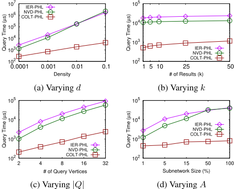
We use the continental US road network that contains 23, 947, 347 vertices and 57, 708, 624 travel time edges combined with 8 real POI sets (see Table 1) for the US from OpenStreetMap provided by [Abeywickrama et al., 2016]. For sensitivity analysis, we generate synthetic POI sets chosen uniformly at random for density d where d=|P |/|V |. We use A to denote a connected subgraph of G with A% of the total vertices |V |. Query vertices are then chosen uniformly at random from the A% subgraph which represents how "local" a group of query locations are [Yiu et al., 2005]. We show the results over 500 queries considering max function. The results for sum can be found in [Abeywickrama et al., 2020].
| Parameter | Values |
|---|---|
| k | 1, 5, 10, 25, 50 |
| d | 1, 0.1, 0.01, 0.001, 0.0001 |
| A (%) | 1, 5, 15, 50, 100 |
| |Q| | 2, 4, 8, 16, 32 |
| Real-World POI Set (|P|) | Schools (160,525), Parks (69,338), Fast Food (25,069), Post Office (21,319), Hospitals (11,417), Hotels (8,742), Universities (3,954), Courthouses (2,161) |
We compare our algorithm against the Incremental Euclidean Restriction (IER) [Yiu et al., 2005] and a concurrent expansion approach which adapts the state-of-the-art kNN heuristic based on Network Voronoi Diagrams (NVDs) [Abeywickrama and Cheema, 2017] for AkNN queries. To ensure fairness, each technique employs Pruned Highway Labeling (PHL) [Akiba et al., 2014], one of the fastest network distance computation techniques, to compute network distances in each approach - hence techniques are named IER-PHL, NVD-PHL, and COLT-PHL. SL-Trees and COLT use branch factor b = 4, maximum object distance list size λ = 128 (which is also α) and m = 4 landmarks per node for ideal performance vs. index size. NVD uses the ALT index [Goldberg and Harrelson, 2005] with m = 16 random landmarks to compute LLBs, which we also use as it is essentially the root of an SL-Tree. All experiments were conducted using memory-resident indexes for fast query processing.
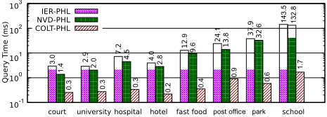
Query performance on real-world data. Figure 3 depicts query time on real-world POI datasets, with the number of objects increasing from left to right. COLT significantly outperforms the other methods across the board, with up to two orders of magnitude improvement. COLT tends to improve more on larger POI sets, where it is more difficult to distinguish between objects.
Query performance on synthetic data. A sensitivity analysis of the query times on the synthetic benchmark sets with respect to the object density d, the value of k, the number of query vertices |Q|, and the percentage A of graph vertices in a subgraph from which we choose query vertices is provided in Figure 4. This reaffirms the observations on real-world data and shows the improvement of COLT is consistent across varying parameters, reaching up to 3 orders magnitude.
| Network Indexes | Obj. Indexes (d=0.001) | |||||
|---|---|---|---|---|---|---|
| ALT | SL-T | PHL | COLT | NVD | R-T | |
| Time | 71s | 25m | 25m | 63ms | 11s | 6ms |
| Space | 1.4GB | 4.6GB | 16GB | 0.9MB | 28MB | 0.9MB |
Preprocessing cost. Table 2 shows preprocessing cost for the road network and object indexes. The SL-Tree consumes greater space than ALT, but not significantly so. Moreover, only the root node of the SL-Tree is required for query processing, which has the same index size as ALT. The indexing time is comparable to PHL, which possesses one of the fastest pre-processing times for high-performance indexes [Akiba et al., 2014]. COLT is significantly smaller and faster to construct than NVDs and is comparable to R-trees as both have space complexity linear to the input.
5 Conclusion
We present two novel light-weight indexes, SL-Tree and COLT, and design an efficient hierarchical traversal algorithm to solve AkNN queries for any convexity preserving aggregate function. Our experiments on real-world and synthetic datasets show that the proposed approach outperforms existing techniques by up to three orders of magnitude.
Acknowledgements
This work was supported by the Australian Research Council (FT180100140 and DP180103411) and the German Research Foundation (SPP 1894, contract number STO 1114/42). Work was mainly completed while Tenindra Abeywickrama was with Monash University.
@inproceedings{ijcai2021p640,
  title     = {Hierarchical Graph Traversal for Aggregate k Nearest Neighbors Search in Road Networks (Extended Abstract)},
  author    = {Abeywickrama, Tenindra and Cheema, Muhammad Aamir and Storandt, Sabine},
  booktitle = {Proceedings of the Thirtieth International Joint Conference on
               Artificial Intelligence, {IJCAI-21}},
  publisher = {International Joint Conferences on Artificial Intelligence Organization},
  editor    = {Zhi-Hua Zhou},
  pages     = {4730--4734},
  year      = {2021},
  month     = {8},
  note      = {Sister Conferences Best Papers},
  doi       = {10.24963/ijcai.2021/640},
  url       = {https://doi.org/10.24963/ijcai.2021/640},
}
TY - CPAPER TI - Hierarchical Graph Traversal for Aggregate k Nearest Neighbors Search in Road Networks (Extended Abstract) AU - Abeywickrama, Tenindra AU - Cheema, Muhammad Aamir AU - Storandt, Sabine T2 - Proceedings of the Thirtieth International Joint Conference on Artificial Intelligence, IJCAI-21 PB - International Joint Conferences on Artificial Intelligence Organization PY - 2021 SP - 4730 EP - 4734 DO - 10.24963/ijcai.2021/640 UR - https://doi.org/10.24963/ijcai.2021/640 ER -Copied
Machine-readable versions of this paper, for tools and AI agents:





