
Traffic Congestion Alleviation over Dynamic Road Networks: Continuous Optimal Route Combination for Trip Query Streams
Proceedings of the Thirtieth International Joint Conference on Artificial Intelligence. Main Track. Pages 3656-3662.
https://doi.org/10.24963/ijcai.2021/503
Keywords
- Multidisciplinary Topics and Applications: Transportation
Abstract
Route planning and recommendation have attracted much attention for decades. In this paper, we study a continuous optimal route combination problem: Given a dynamic road network and a stream of trip queries, we continuously find an optimal route combination for each new query batch over the query stream such that the total travel time for all routes is minimized. Each route corresponds to a planning result for a particular trip query in the current query batch. Our problem targets a variety of applications, including traffic-flow management, real-time route planning and continuous congestion prevention. The exact algorithm bears exponential time complexity and is computationally prohibitive for application scenarios in dynamic traffic networks. To address this problem, a self-aware batch processing algorithm is developed in this paper. Extensive experiments offer insight into the accuracy and efficiency of our proposed algorithms.
- [Babak et al., 2018] Javani Babak, Babazadeh Abbas, and Ceder Avishai (Avi). Path-based capacity-restrained dy- namic traffic assignment algorithm. Transportmetrica B: Transport Dynamics, pages 1-24, 2018.
- [Cao et al., 2012] Xin Cao, Lisi Chen, Gao Cong, and Xi- aokui Xiao. Keyword-aware optimal route search. Proc. VLDB Endow., 5(11):1136-1147, 2012.
- [Chen et al., 2010] Zaiben Chen, Heng Tao Shen, Xiaofang Zhou, Yu Zheng, and Xing Xie. Searching trajectories by locations: an efficiency study. In SIGMOD Conference, pages 255-266. ACM, 2010.
- [Chen et al., 2019] Lisi Chen, Shuo Shang, Christian S. Jensen, Bin Yao, Zhiwei Zhang, and Ling Shao. Effec- tive and efficient reuse of past travel behavior for route recommendation. In KDD, pages 488-498. ACM, 2019.
- [Chen et al., 2020a] Lisi Chen, Shuo Shang, and Tao Guo. Real-time route search by locations. In AAAI, pages 574- 581. AAAI Press, 2020.
- [Chen et al., 2020b] Lisi Chen, Shuo Shang, Bin Yao, and Jing Li. Pay your trip for traffic congestion: Dynamic pricing in traffic-aware road networks. In AAAI, pages 582-589. AAAI Press, 2020.
- [Dafermos and C., 1972] Dafermos and Stella C. The traf- fic assignment problem for multiclass-user transportation networks. Transportation Science, 6(1):73-87, 1972.
- [Dijkstra, 1959] Edsger Wybe. Dijkstra. A note on two prob- lems in connexion with graphs. Numerische Mathematik, 1:269-271, 1959.
- [Greenshields, 1934] B. Greenshields. A study of traffic ca- pacity. A Study of Traffic Capacity, 14, 01 1934.
- [Guo et al., 2018] Chenjuan Guo, Bin Yang, Jilin Hu, and Christian S. Jensen. Learning to route with sparse tra- jectory sets. In ICDE, pages 1073-1084. IEEE Computer Society, 2018.
- [Li et al., 2013] Jing Li, Yin David Yang, and Nikos Mamoulis. Optimal route queries with arbitrary order con- straints. IEEE Trans. Knowl. Data Eng., 25(5):1097-1110, 2013.
- [Li et al., 2020] Ke Li, Lisi Chen, and Shuo Shang. Towards alleviating traffic congestion: Optimal route planning for massive-scale trips. In IJCAI, pages 3400-3406. ijcai.org, 2020. IJCAI
- [Liebig et al., 2017] Thomas Liebig, Nico Piatkowski, Christian Bockermann, and Katharina Morik. Dynamic route planning with real-time traffic predictions. Inf. Syst., 64:258-265, 2017.
- [Lim and Rus, 2012] Sejoon Lim and Daniela Rus. Stochas- tic distributed multi-agent planning and applications to traffic. ICRA, pages 2873-2879, 2012.
- [Malviya et al., 2011] Nirmesh Malviya, Samuel Madden, and Arnab Bhattacharya. A continuous query system for dynamic route planning. In ICDE, pages 792-803. IEEE Computer Society, 2011. Shang et al., 2012]
- Shuo Shang, Ruogu Ding, Bo Yuan, Kexin Xie, Kai Zheng, and Panos Kalnis. User oriented trajectory search for trip recommendation. In EDBT '12, Berlin, Germany, March 27-30, 2012, Proceedings, pages 156-167. ACM, 2012.
- [Shang et al., 2013] Shuo Shang, Hua Lu, Torben Bach Ped- ersen, and Xike Xie. Modeling of traffic-aware travel time in spatial networks. In MDM (1), pages 247-250. IEEE Computer Society, 2013.
- [Shang et al., 2014] Shuo Shang, Ruogu Ding, Kai Zheng, Christian S. Jensen, Panos Kalnis, and Xiaofang Zhou. Personalized trajectory matching in spatial networks. VLDB J., 23(3):449-468, 2014.
- [Shang et al., 2015] Shuo Shang, Jiajun Liu, Kai Zheng, Hua Lu, Torben Bach Pedersen, and Ji-Rong Wen. Plan- ning unobstructed paths in traffic-aware spatial networks. GeoInformatica, 19(4):723-746, 2015.
- [Shang et al., 2016] Shuo Shang, Lisi Chen, Zhewei Wei, Christian S. Jensen, Ji-Rong Wen, and Panos Kalnis. Col- lective travel planning in spatial networks. IEEE Trans. Knowl. Data Eng., 28(5):1132-1146, 2016.
- [Shang et al., 2017] Shuo Shang, Lisi Chen, Christian S. Jensen, Ji-Rong Wen, and Panos Kalnis. Searching tra- jectories by regions of interest. IEEE Trans. Knowl. Data Eng., 29(7):1549-1562, 2017.
- [Shang et al., 2019] Shuo Shang, Lisi Chen, Kai Zheng, Christian S. Jensen, Zhewei Wei, and Panos Kalnis. Par- allel trajectory-to-location join. IEEE Trans. Knowl. Data Eng., 31(6):1194-1207, 2019.
- [Sharifzadeh et al., 2008] Mehdi Sharifzadeh, Moham- mad R. Kolahdouzan, and Cyrus Shahabi. The optimal sequenced route query. VLDB J., 17(4):765-787, 2008.
- [Wilkie et al., 2011] David Wilkie, Jur P. van den Berg, Ming C. Lin, and Dinesh Manocha. Self-aware traffic route planning. In AAAI. AAAI Press, 2011.
- [Xu et al., 2012] Jiajie Xu, Limin Guo, Zhiming Ding, Xil- ing Sun, and Chengfei Liu. Traffic aware route planning in dynamic road networks. In DASFAA (1), volume 7238 of Lecture Notes in Computer Science, pages 576-591. Springer, 2012.
- [Zeng et al., 2015] Yifeng Zeng, Xuefeng Chen, Xin Cao, Shengchao Qin, Marc Cavazza, and Yanping Xiang. Op- timal route search with the coverage of users' preferences. In IJCAI, pages 2118-2124. AAAI Press, 2015. IJCAI
References were extracted automatically from the PDF and may contain errors.
Full text extracted automatically from the PDF; figures, tables and equations may differ. The PDF is the version of record.
1 Introduction
With the growing popularity of location-based services, many route planning services (e.g., Google Maps) and ridesharing services (e.g., DiDi, Uber, and Grab) are playing an indispensable role in our lives. Route planning and recommendation have attracted much attention in recent years [Sharifzadeh et al., 2008; Shang et al., 2013; Li et al., 2013; Zeng et al., 2015; Shang et al., 2019]. Some studies focus on the optimal route planning for a single trip query under current traffic condition (e.g., [Malviya et al., 2011]).
As route planning services and ridesharing services are becoming increasingly popular, massive-scale users in a city may issue trip queries within a short period of time, especially during rush hours. Thus, it is of great importance to enable route planning for a stream of trip queries based on realtime traffic conditions. Existing related proposals aim to find an optimal route (i.e., a route with the minimum travel time) for each single trip [Malviya et al., 2011; Xu et al., 2012; Shang et al., 2012; Shang et al., 2015]. However, recommending the optimal route based on individual trip query may induce potential traffic congestion. Recently, [Li et al., 2020] recognizes this potential traffic congestion and studies the problem of finding a route for each trip such that the global travel time cost for all trips is minimized. However, it only considers a static collection of trip queries as input, making it ineffective to handle a stream of trip queries in practice as the routes recommended ahead of current time are ignored. As a result, its solutions cannot be used to answer continuous trip queries in practice.
∗Corresponding author
In this light, we study a Continuous Optimal Route Combination (CORC) problem: Given a dynamic road network G and a stream of trip queries Q={q1, q2, . . .}, we aim to periodically generate an optimal route combination Π={π1, π2, . . .} for new trip queries such that the total travel time of all routes in Π is minimized. In our settings, the realtime travel time on each edge e is proportional to the number of current vehicles on e. The problem is challenging due to its high computational cost. The time complexity of the exact algorithm is exponential to the number of queries, thus it is impossible to find the optimal route combination in interactive time. To enable high efficiency, a self-aware batch process algorithm (SBP) and its corresponding pruning techniques are developed. In addition to the non-query traffic flow and the query-related flow caused by our planned routes ahead of current time, we also consider the potential traffic flow caused by those planning initial routes. The main contributions of this paper can be summarized as follows.
- We propose a novel CORC problem that targets a variety of applications, including traffic-flowmanagement, realtime route planning and congestion prevention.
- We develop a self-aware batch process algorithm (SBP) for answering CORC problem.
- The accuracy and efficiency of our solutions are evaluated by extensive experiments over two real-life datasets. The experimental results show that our proposal outperforms the baseline method and it is capable of handling streams of trip queries in real-time fashion.
Related work. Optimal route planning is extensively investigated under different settings [Shang et al., 2016; Guo et al., 2018; Chen et al., 2019; Chen et al., 2020a; Chen et al., 2020b]. Some studies aim to generate a route based on a particular optimization goal (e.g., the shortest distance, minimum congestion probability) under user-specified constraints (e.g., the departure time) [Chen et al., 2010; Cao et al., 2012; Shang et al., 2014; Liebig et al., 2017]. However, such queries proposed by these studies are based on a singe trip. Existing studies of traffic-based global optimization problems [Dafermos and C., 1972; Lim and Rus, 2012; Babak et al., 2018] can be regarded as the flow assignment problem rather than real-time route planning problem, where the routes are pre-defined and they search for an optimal flow assignment to each route. Though a recent work [Li et al., 2020] proposes to minimize the global travel time, its solutions cannot be used to answer CORC problem. The reason we have explained in introduction.
2 Preliminaries and Problem Statement
Dynamic road networks. We formulate a dynamic road network by a connected and directed graph G(V,E), which consists of a set of vertexes V representing road intersections or ends, and edges E ⊂ V × V representing road segments. Each edge e(vi, vj) ∈ E connects two end-points vi and vj where vi, vj ∈ V . Associated with each road segment e is a natural-valued road capacity Ce and a minimum travel time Tm(e), denoting the travel time on e when there are no vehicles. 1 The dynamic weight of an edge e, denoted by T(e, t), is the travel time for passing through e, which is at least Tm(e) and is proportional to the number of current vehicles on e.
Travel time function. The travel time of a vehicle on road segment e at time t is correlated to current number of vehicles, which is defined as traffic flow [Greenshields, 1934]. Following existing studies [Lim and Rus, 2012; Babak et al., 2018; Li et al., 2020], we use a popular travel time function (cf. Equation 1) based on current traffic flow on e (i.e., f(e, t)) to compute the estimated travel time of segment e at time t, which is denoted by T(e, t). Here, Ce is the capacity of segment e, α and β are road-specific parameters, which are determined by segment attributes (e.g., speed limit, road width). Note that our proposal is independent of these parameters. Our modeling of road networks aligns with existing studies [Wilkie et al., 2011; Shang et al., 2017; Chen et al., 2020b].
Route and its estimated travel time. Route π is defined as a finite sequence of vertices 〈v0, v1, . . . , v|π|-1〉. Assume that route π starts at time t0 and ti is the estimated arrival time on vertex vi (i.e., ti = ti-1 + T(e(vi-1, vi), ti-1)). Denoted by ET(π, t0) the estimated travel time of π departing at time t0 is computed by the sum of estimated travel times on each road segment traveled by π (cf. Equation 2). In remaining parts of this paper, we use π.v0 and π.v|π|-1 to denote the first and the last vertices of π, respectively.
1 For ease of presentation, we use e to represent e(vi, vj) where the context is clear.
Trip query stream. A single trip query is denoted by q = (s, d, t), where s is the source location, d is the destination location, and t is the departure time. Q = {q1, q2, . . .} denotes a stream of trip queries arriving in a streaming manner (i.e.,∀qi, qj ∈ Q, i > j: qi.t ≥ qj.t). Note that Q is dynamically updated by new trip queries over the data stream.
Continuous Optimal Route Combination (CORC) Problem. Given a dynamic road network G, a stream of trip queries Q = {q1, q2, . . .}, and a time interval T, the CORC problem aims to process the newly issued query batch Qn = {qk, qk+1, . . . , q|Q|} (Qn ⊂ Q ∧ q|Q|.t - qk.t = T) for an optimal route combination Π = {π1, π2, . . .} such that:
- |Q| = |Π|;
- (∀πi ∈ Π) (πi.v0 = qi.s ∧ πi.v|πi|-1 = qi.d);
- The sum of estimated travel time for routes in Π, denoted by TT(Π) (cf. Equation 3), is minimized.
3 Exact Traversal Algorithm
An exact method for answering the CORC problem works as follows: for each incoming trip query q ∈ Q, we first run Depth-First Search (DFS) on the road network to find all possible routes from q.s to q.d. Next, we evaluate all possible route combinations and select the combination that has the minimum TT(Π) as result. To answer the CORC problem in a real-time fashion, exact traversal algorithm (ETA) periodically conducts aforementioned operations to return an optimal combination as real-time result. If the number of possibles routes for each query is k and there are totally |Q| trip queries, the ETA will performs exhaustive evaluation of k|Q| possible route combinations.
4 Self-Aware Batch Processing Algorithm
To answer the CORC problem efficiently, we propose a Selfaware Batch Processing (SBP) algorithm, which consists of two primary steps: (1) Initial Route Search and (2) Batch Refining Processing. In particular, given a batch of new trip queries Qn, we first run Initial Route Search that generates an high-quality initial route combination Πn consisting of planned routes for each incoming trip query. Next, we run Batch Refining Processing to refine the routes in Πn.
In remaining parts of this section, we present Initial Route Search and Self-Aware Batch Refining algorithms. Finally, we present an overall solution based on the self-aware batch processing algorithm.
4.1 Initial Route Search
The objective of Initial Route Search is to generate a highquality individual route for each trip query q in a new query batch Qn. The time-aware traffic flow is calculated as a combination of "query-related flow" and "other traffic flow". Specifically, the query-related flow is the extra traffic flow incurred by routes planned for queries in Q, which is selfaware. The other traffic flow is resulted from traffic flow outside Q. We take other traffic flow directly as input.
Algorithm 1 InitSearch (G, q, L)
Input: Dynamic road network G = (V, E); A trip query q = (vs, vd, t); All-pair lower-bound estimation for the travel time H(vi, vj ); A set of edge labels L of planned routes; Output: An initial route π for query q; 1: Init: ∀v ∈ V : v.ts =∞, v.td =H(v, vd), v.et = t;vs.pred = null, vs.ts = 0; π = ∅; 2: PQ← {vs}; 3: while PQ ̸= ∅ do 4: v ←PQ.pop(); 5: if v = vd then 6: while vd.pred ̸= null do 7: π ← {vd, π}; 8: vd ← vd.pred; 9: end while 10: return π; 11: end if 12: for each edge e(v, v′ ) ∈ G do 13: calculate the current traffic flow f(e, v.et); 14: if v.ts +T(e, v.et) ≤ v′ .ts then 15: v′ .ts ← v.ts + T(e, v.et); 16: v′ .et ← t + v′ .ts; 17: v′ .pred ← v; 18: if v′ /∈ PQ then 19: PQ.push(v′ ); 20: end if 21: end if 22: end for 23: end whileEdge labels. To enable fast computation of the traffic flow on each edge caused by planned routes, we maintain a label Le = {l1, l2, . . .} for each edge e to record the time information of each route that travels on e. A label li = {ta, tb} consists of the timestamp entering e (i.e., ta) and the timestamp leaving e (i.e., tb) of a route. Initially, the Le of each edge is empty and they are dynamically updated each time we complete the processing of a new batch of trip queries.
Query-Related flow calculation. The query-related flow on edge e at timestamp t is the number of edge label li ∈ Le that satisfies [li.ta, li.tb] ∋ t. A priority queue is applied to accelerate computation in our experiment study.
Lower-bound Travel Time Estimation We use a heuristic value H(vi, vj) to denote the lower-bound estimation of the travel time from vertex vi to vj , it is pre-computed by Dijkstra [Dijkstra, 1959] given the minimum non-query flow. Note that the minimum non-query flow on each edge e is regarded as a static value. We take it directly as input.
Algorithm description. Algorithm 1 presents the pseudo code of Initial Route Search. The input includes a dynamic road network G = (V,E), a trip query q = (vs, vd, t), allpairs lower-bound travel time H(vi, vj), and a collection of edge label sets L = {Le1 ,Le2 , ...} consisting of edge label set Le for each edge e. The output is an initial route planned for q. Associated with each v ∈ V is the exact travel time from q.vs to v, which is denoted by ts; a heuristic value td representing the lower-bound travel time from v to the destination q.vd; the earliest arriving time of v from vs to v, which is denoted by et; and a predecessor pred. First, we initialize each v ∈ V and set the route π a empty set (line 1). Then we add the starting vertex vs into the priority queue PQ that sorts vertexes in ascending order based on v.ts+v.td (line 2). During the search process, in each iteration we select a vertex v from PQ and explore its adjacent vertices (lines 3-23). To be specific, each time we select the v with minimum v.ts + v.td on the top of PQ, which is based on the hypothesis that this v may be a intermediate destination with minimum travel time cost (line 4). If v is the destination, we utilize the predecessor record pred of corresponding vertexes to generate a route π as the result (lines 5-11). If v is not the destination, for each edge e starting from v, we calculate the current traffic flow on e(line 13). For the ending vertex v′ of e(v, v′ ), we check whether it can be reached with a smaller ts through vertex v (line 14). If it satisfies we will update ts, et and pred of v′ , respectively (lines 15-17). In the next, we add v′ into PQ for next iteration if v′ is not contained in PQ. The algorithm terminates when PQ is empty or the destination is found. In the worst case, we need to evaluate all vertexes. The maximum number of adjacent vertices of a vertex is up to |V |, thus the maximum times of edge evaluation is |V |2 . Computing the query-related flow on edge e requires time complexity O(|Le|). Assume the maximum value of O(|Le|) is m, the total time complexity of the Initial Route Search is O(m|V |2 ).
4.2 Batch Refining Processing
To improve the result quality, a Batch Refining Processing method is developed to refine these initial routes Πn of Qn (cf. Algorithm 1). We reuse the initial route combination Πn and refine each πi ∈ Πn with a self-aware swapping strategy in a batch mode. The high-level idea works as follows: During each refinement we select a route πi ∈ Πn, then we take other planning initial routes (i.e, Πn \ πi) as known traffic flow input to re-predict the traffic condition and reassign a route π′i to qi. Note that the swap operation is performed for a whole route. We swap π ∈ Πn with π′ , denoted by Πn.swap(π, π′ ). If this swapping operation can reduce the total travel time of all trips at least by a factor of 1 + ϵ (e.g., T T ({Π,Πn}) TT({Π,Πn.swap(π,π′ )}) > (1 + ϵ), we define this swapping operation as a valid operation and apply it. Here, the small constant ϵ is used to filter out some "useless" operations (i.e., the operations that only reduce little travel time) and guarantee the number of swapping operations is finite.
Swapping operation. During our refining process, in addition to the non-query traffic flow and the query-related flow caused by our planned routes ahead of current time, we also consider the potential traffic flow caused by planning initial routes. A new edge label L′ = {L,L(Πn \ πi)} is defined as a combination of primitive edge labels L and the estimated time information of these planning initial routes in Πn except route πi (cf. Algorithm 1). We reassign a new route π′i to qi by conducting Algorithm 1 that uses L′ as traffic condition input, and we will swap πi ∈ Πn by π′i if it is valid.
Algorithm 2 BatchRefining(G, Π, Πn, L, ϵ)
Input: Dynamic road network G = (V, E), The global route combination Π , An initial route combination Πn, A set of edge labels L of planned routes, Parameter ϵ Output: A refined route combination Πn 1: Init:flag ← true; 2: while flag do 3: flag ← false; 4: for each route πi ∈ Πn do 5: if UB(πi) > (1 + ϵ) then 6: L′ ← {L, L(Πn \ πi)}; 7: π′ ← InitSearch(G, qi, L′ ); 8: if the operation Πn.swap(π, π′ ) is valid then 9: Πn ← Πn.swap(π, π′ ); 10: f lag ← true; 11: end if 12: end if 13: end for 14: end while 15: return ΠnPre-checking strategy. In order to check whether the swapping operation is valid, we have to update the edge labels of all edges to calculate the ratio of decreased travel time, which is time-consuming. Here, a pre-checking strategy is developed to improve efficiency. In Equation 4, we define an upper bound UB as the maximum ratio of decreased travel time of refining route π ∈ Πn. Note that TT({Π, Πn \ π}) ̸= TT({Π, Πn}) - ET(π, t), here TT({Π, Πn \ π}) is the total travel time assuming that route π does not exist. In such case the extra increased travel time of other routes caused by route π should be excluded in addition to the travel time of the route π itself.
Algorithm description. Algorithm 2 presents the pseudo code of our Batch Refining Processing method. Initially, we use a flag to mark if any valid swapping operation applied in last "while" loop and we initially set it true (line 1). During the refining process, for each initial route π ∈ Πn we check whether it could be swapped by a new route π′ (lines 4-13). Specifically, we first change the flag to assume there is no valid swapping operation in current "while" loop (line 3). For each π ∈ Πn, we compute the UB(π) to determine whether the operation is possibly valid (line 5). If it is possibly valid, we generate a new edge labels L′ by combining the primitive edge label L and the traffic flow caused by the currently planning routes in Πn except the πi itself (line 6). Then given the L′ as input we generate a new route π′ by conducting Algorithm 1 (line 7). In the next, we apply the swapping operation if π′ ̸= π and the exact total travel time decreased by at least a factor of 1+ϵ through this swapping, then we set flag true again to record the fact that there are valid swapping operations applied (lines 8-11). The algorithm terminates when no
Algorithm 3 SBP(G, Q, T, ϵ)
Input: Dynamic road network G = (V, E), a stream of trip queries Q, Refining Interval T , Parameter ϵ Output: A real-time route combination Π 1: Init: L← ∅;Π← ∅; Πn ← ∅ 2: while true do 3: for each incoming trip query q ∈ Q do 4: π ← InitSearch(G, q, L); 5: Πn ← {Πn, π}; 6: end for 7: if currentTime %T = 0 then 8: Πn ←BatchRefining(G,Π,Πn,L, ϵ); 9: Π← {Π,Πn}; 10: L← {L,L(Πn)}; 11: Πn ← ∅; 12: Output Π as real-time result 13: end if 14: end whilevalid swapping operations applied during current loop for all π ∈ Πn, indicating that no valid swapping operation could produce a better result.
4.3 Overall Solution for CORC Problem
By integrating all above methods, here we present the SBP algorithm for answering the CORC problem.
Refining interval. In our settings, the Batch Refining Processing (cf. Algorithm 2) is periodically conducted at a fixed frequency (e.g., 2s). We define T as the time interval between each two batch refining operations. By utilizing the refining interval T, we can more accurately predict future traffic condition for more planning initial routes are considered as known traffic flow input, thus we can reduce the TT(Π) more by a valid swapping operation, which enables less swapping operations occurred during the whole refining process.
Algorithm descriptions. The overall solution of the SBP Algorithm for CORC problem is presented in Algorithm 3. Initially, there are no trip queries in our query system. We set the edge labels L and the global route combination Π a empty set, which records the planned routes of all trip queries. We use a route combination Πn to store the planning initial routes of a new query batch Qn, initially it is empty (line 1). First we perform Algorithm 1 to generate an initial route π for each new trip query q ∈ Q (lines 3-6). We perform aforementioned operations until the time-up for next Batch Refining Processing (line 7). During the refinement, we conduct Algorithm 2 to generate a refined Πn (line 8). In the next, we add these refined routes into the global route combination Π and update the edge labels L accordingly (lines 9-10). At the end of each refinement, since all initial routes have been refined, we reset the Πn empty (line 11). The empty Πn is used to store new initial routes that planned for next batch of trip queries subsequently. We output the global route combination Π as real-time result each time we complete the refining processing of a new batch of trip queries (line 12).
| TG | NY | |
|---|---|---|
| Number of queries |Q| | 4,000-20,000 /default 4,000 | 2,000-10,000 /default 2,000 |
| Parameter ϵ | 0.0002-0.0010 /default 0.001 | 0.0002-0.0010 /default 0.001 |
| Refining interval T | 1s-5s /default 2s | 1s-5s /default 2s |
| Query arrival rate | 20/s-100/s /default 50/s | 20/s-100/s /default 50/s |
| α (cf. Equation 1) | 1-5 /default 2 | 1-5 /default 2 |
| β (cf. Equation 1) | 1-3 /default 2 | 1-3 /default 2 |
5 Experimental Study
5.1 Experimental Settings
Datasets. Two real road networks are used in our experimental study: San Joaquin County Road Network (TG) 2 and the New York Road Network (NY) 3 ,which contain 18,263 vertices and 23,874 edges, and 95,581 vertices and 260,855 edges, respectively. A capacity Ce ranging form 20 to 100 was assigned to each road segment based on the road length for both TG and NY. The minimum travel time Tm(e) is a randomly generated value ranging from 5 to 10 (minutes) for each edge. To simulate the non-query vehicles, we assume the averaged traffic flow ¯x of non-query vehicles on edge e is 0.4 × Ce, and the number of real-time non-query vehicles on edges cyclically change by a ratio ranging from 0.8¯x to 1.2¯x over time. Given traffic flows 0.8¯x on all road segments, we pre-compute the all-pair minimum travel time using Dijkstra algorithm [Dijkstra, 1959] and store the results. We generate a stream of trip queries by randomly sampling source-destination pairs in those areas with high density of road intersections (e.g., the mean out-degree of the area is no less than 3), which is consistent with the real-life application scenarios. Given a departure time q1.t of the first trip, the departure time of subsequent trips increase by a short period of time. The query arrival rate setting is presented in Table 1.
Computing traffic flow. The real-time traffic flow f(e, t) on edge e at timestamp t, is computed by Equation 5. Here, f ′ (e, t) denotes the number of non-query vehicles, while f ′′ (e, t) is the number of vehicles using our query system. To simulate the non-query vehicles, we assume f ′ (e, t) cyclically change (e.g.,f ′ (e, t + T)=f ′ (e, t) ,T=2h) over time. How to calculate f ′′ (e, t) is detailed in Algorithm 1.
Evaluation settings. To evaluate the result quality of SBP algorithm, we implement an individual-based search algorithm (Ind algorithm). Specifically, given a stream of trip queries Q, for each trip q ∈ Q we derive a route π with the minimum travel time ET(π, q.t) regrading current traffic condition at timestamp q.t, which aligns with existing works [Malviya et al., 2011; Xu et al., 2012]. Note that the exact algorithm is extremely time-consuming, which requires at least 1 day with default setting. Thus, we do not report its performance. To evaluate the performance of our Initial Route Search method that takes self-awareness and network dynamics into account, we implement SBP*SA algorithm and SBP*DA algorithm, respectively. Here, the SBP*SA is the SBP algorithm without self-aware idea. Specifically, it applies an Initial Route Search method that is not aware of extra traffic flow caused by planned routes. The SBP*DA is the SBP algorithm with the assumption that the traffic flow is static. In particular, it generates initial routes regrading a snapshot of traffic condition at the departure time of each trip. The performance metrics for efficiency evaluation and efficacy evaluation are CPU time and the total travel time TT(Π) of the route combination Π generated by the proposed algorithm, respectively. All algorithms were conducted in Java and tested on a Windows 10 platform with Intel(R) i5-9300H CPU (2.40 GHz) and 16GB memory. The default parameter settings are listed in Table 1.
2 https://www.cs.utah.edu/∼lifeifei/SpatialDataset.htm
3 https://publish.illinois.edu/dbwork/open-data/
5.2 Experimental Results
Effect of the number of trip queries. First, we investigate the effect of the query count |Q| on the performance of the proposed algorithms with the default setting. Intuitively, a larger |Q| leads to the increment of the total travel time. Additionally, a larger |Q| causes more computation effort for evaluating more edges and the CPU time is thus increased. Figure 1 shows the performance of the proposed algorithms in TG and NY, respectively. As expected, the CPU time increases when |Q| become larger for all algorithms. Among these algorithms, the Ind algorithm requires less CPU time because it is a one-time planning mechanism without refining process. Compared with Ind algorithm, SBP algorithm can reduce at least 40% total travel time. SBP*SA and SBP*DA perform slightly worse than SBP since more swapping operations performed in their refining process. Particularly, the SBP*SA does not consider the traffic flow caused by these planned routes, thus making traffic prediction insufficiently. SBP*DA plans initial routes regarding the static traffic flow at the departure time. Hence, the initial routes planned by SBP*SA and SBP*DA are of low-quality, which leads to more refining effort to improve result quality. We also observe that the results of the three algorithms are reasonably close , as shown in Figure 1(b) and Figure 1(d), and SBP consistently exhibits less total travel time. These results demonstrate the superiority of our Initial Route Search.
Effect of the query arrival rate. A larger query arrival rate indicates that more vehicles are coming to roads per unit time. In such case, the increment of traffic flow on edges exhibits more significant. Consequently, there will be more extra traffic flow caused by planned routes on each road. In Figure 2, an increasing trend regarding the CPU time and TT(Π) is observed in both NY and TG. Here, the CPU time increases for more swapping operations are conducted in refining process to further alleviate traffic congestion. And the TT(Π) increases for traffic flow of edges increase accordingly, more travel time is thus required to pass through an edge. Note that the SBP Algorithm results in a larger TT(Π) in TG than that in NY for we process more trip queries in TG by default.
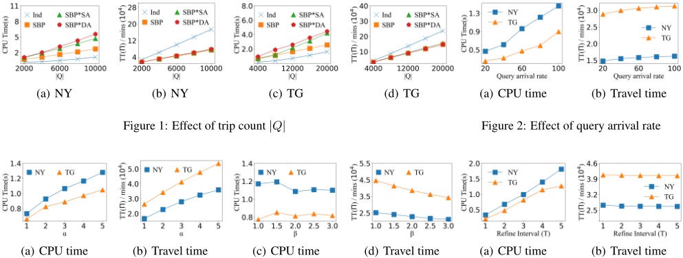
Figure 4: Effect of refining interval T
Effect of the parameters of travel time function. Figure 3 shows the performance of the SBP algorithm as we vary the parameters α and β (cf. Equation 1). Intuitively, a larger α or a smaller β leads to more traffic congestion because that more travel time is required to pass through an edge. In Figure 3, an increasing trend regarding both CPU time and the TT(Π) is observed as we vary α from 1 to 5. In contrast, the travel time decreases as we vary β from 1.0 to 3.0. It's worth noting that there are no specific trend regarding CPU time as we vary β for CPU time is not directly related to the value of β.
Effect of the refining interval. A larger value of refining interval T denotes that the waiting time for each query is increased while the planning results are closer to the optimal result because more planed routes are considered. In such case, we are able to substantially reduce the TT(Π) through swapping operations. From Figure 4(a), we see that the CPU time increases as T increases, the reason is that we process more trip queries in each refinement. A slightly decreasing trend of TT(Π) is observed in Figure 4(b). These results demonstrate that an appropriate T is helpful to avoid traffic congestion by reusing planning initial routes to more accurately predict future traffic condition.
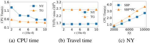
Effect of ϵ and pre-checking strategy. We study the effect of the refining parameter ϵ. A larger ϵ means fewer valid operations (cf. Algorithm 3), thus less CPU time is required. However, a larger ϵ also results in a route combination Π with a larger TT(Π). As we vary ϵ from 0.0002 to 0.001, a decreasing trend of CPU time is observed in Figure 5(a). In contrast, a slightly increasing trend of TT(Π) is observed in Figure 5(b). Note that the CPU time decreases rapidly when we vary ϵ from 0.0002 to 0.0004. It is worth noting that the TT(Π) slightly increases as ϵ increases. We also find that 0.001 is an optimal value of ϵ that enables both high efficiency and effectiveness. The SBP algorithm without pre-checking strategy is denoted by "SBP*PC". In Figure 5(c), we observe that the required CPU time of SBP is consistently less than those of SBP*PC, which shows that our pre-checking strategy is able to enhance efficiency.
6 Conclusions
We proposed and investigated a novel route planning problem that finds optimal route combination for a stream of trip queries (CORC problem). The SBP algorithm was proposed for answering CORC problem efficiently. Pruning techniques were developed to enhance efficiency. Extensive experiments confirmed that our proposal was capable of achieving high efficiency and high effectiveness, and the pre-checking strategy was helpful to avoid unnecessary computation.
Acknowledgments
Ke Li and Shuo Shang were supported by the NSFC (U2001212, 62032001, and 61932004). Bin Yao was supported by the NSFC (61922054, 61872235, 61832017, and 61729202), and the National Key Research and Development Program of China (2020YFB1710202, and 2018YFC1504504).
@inproceedings{ijcai2021p503,
  title     = {Traffic Congestion Alleviation over Dynamic Road Networks: Continuous Optimal Route Combination for Trip Query Streams},
  author    = {Li, Ke and Chen, Lisi and Shang, Shuo and Kalnis, Panos and Yao, Bin},
  booktitle = {Proceedings of the Thirtieth International Joint Conference on
               Artificial Intelligence, {IJCAI-21}},
  publisher = {International Joint Conferences on Artificial Intelligence Organization},
  editor    = {Zhi-Hua Zhou},
  pages     = {3656--3662},
  year      = {2021},
  month     = {8},
  note      = {Main Track},
  doi       = {10.24963/ijcai.2021/503},
  url       = {https://doi.org/10.24963/ijcai.2021/503},
}
TY - CPAPER TI - Traffic Congestion Alleviation over Dynamic Road Networks: Continuous Optimal Route Combination for Trip Query Streams AU - Li, Ke AU - Chen, Lisi AU - Shang, Shuo AU - Kalnis, Panos AU - Yao, Bin T2 - Proceedings of the Thirtieth International Joint Conference on Artificial Intelligence, IJCAI-21 PB - International Joint Conferences on Artificial Intelligence Organization PY - 2021 SP - 3656 EP - 3662 DO - 10.24963/ijcai.2021/503 UR - https://doi.org/10.24963/ijcai.2021/503 ER -Copied
Machine-readable versions of this paper, for tools and AI agents:





