
Hyperspectral Band Selection via Spatial-Spectral Weighted Region-wise Multiple Graph Fusion-Based Spectral Clustering
Proceedings of the Thirtieth International Joint Conference on Artificial Intelligence. Main Track. Pages 3038-3044.
https://doi.org/10.24963/ijcai.2021/418
Keywords
- Machine Learning: Unsupervised Learning
- Machine Learning Applications: Applications of Unsupervised Learning
Abstract
In this paper, we propose a hyperspectral band selection method via spatial-spectral weighted region-wise multiple graph fusion-based spectral clustering, referred to as RMGF briefly. Considering that different objects have different reflection characteristics, we use a superpixel segmentation algorithm to segment the first principal component of original hyperspectral image cube into homogeneous regions. For each superpixel, we construct a corresponding similarity graph to reflect the similarity between band pairs. Then, a multiple graph diffusion strategy with theoretical convergence guarantee is designed to learn a unified graph for partitioning the whole hyperspectral cube into several subcubes via spectral clustering. During the graph diffusion process, the spatial and spectral information of each superpixel are embedded to make spatial/spectral similar superpixels contribute more to each other. Finally, the band containing minimum noise in each subcube is selected to represent the whole subcube. Extensive experiments are conducted on three public datasets to validate the superiority of the proposed method when compared with other state-of-the-art ones.
- [Bai et al., 2017] Song Bai, Xiang Bai, Qi Tian, and Lon- gin Jan Latecki. Regularized diffusion process for visual retrieval. In AAAI, pages 3967-3973, 2017.
- [Bandos et al., 2009] Tatyana V Bandos, Lorenzo Bruzzone, and Gustavo Camps-Valls. Classification of hyperspectral images with regularized linear discriminant analysis. IEEE TGARS, 47(3):862-873, 2009.
- [Cao et al., 2019] Xianghai Cao, Cuicui Wei, Yiming Ge, Jie Feng, Jing Zhao, and Licheng Jiao. Semi-supervised hy- perspectral band selection based on dynamic classifier se- lection. IEEE JSTARS, 12(4):1289-1298, 2019.
- [Chang and Wang, 2006] Chein-I Chang and Su Wang. Con- strained band selection for hyperspectral imagery. IEEE TGARS, 44(6):1575-1585, 2006.
- [Chang et al., 1999] Chein-I Chang, Qian Du, Tzu-Lung Sun, and Mark LG Althouse. A joint band prioritiza- tion and band-decorrelation approach to band selection for hyperspectral image classification. IEEE TGARS, 37(6):2631-2641, 1999.
- [Donoser and Bischof, 2013] Michael Donoser and Horst Bischof. Diffusion processes for retrieval revisited. In CVPR, pages 1320-1327, 2013.
- [Du et al., 2003] Hongtao Du, Hairong Qi, Xiaoling Wang, Rajeev Ramanath, and Wesley E Snyder. Band selection using independent component analysis for hyperspectral image processing. In AIPRW, pages 93-98. IEEE, 2003.
- [Feng et al., 2014] Jie Feng, Licheng Jiao, Fang Liu, Tao Sun, and Xiangrong Zhang. Mutual-information-based semi-supervised hyperspectral band selection with high discrimination, high information, and low redundancy. IEEE TGARS, 53(5):2956-2969, 2014.
- [Geng et al., 2014] Xiurui Geng, Kang Sun, Luyan Ji, and Yongchao Zhao. A fast volume-gradient-based band s- election method for hyperspectral image. IEEE TGARS, 52(11):7111-7119, 2014.
- [Goetz, 2009] Alexander FH Goetz. Three decades of hy- perspectral remote sensing of the earth: A personal view. Remote Sensing of Environment, 113:S5-S16, 2009.
- [Green et al., 1988] Andrew A Green, Mark Berman, Paul Switzer, and Maurice D Craig. A transformation for or- dering multispectral data in terms of image quality with implications for noise removal. IEEE TGARS, 26(1):65- 74, 1988.
- [Guo et al., 2006] Baofeng Guo, Steve R Gunn, Robert I Damper, and James DB Nelson. Band selection for hy- perspectral image classification using mutual information. IEEE GRSL, 3(4):522-526, 2006.
- [Jia et al., 2012] Sen Jia, Zhen Ji, Yuntao Qian, and Linlin Shen. Unsupervised band selection for hyperspectral im- agery classification without manual band removal. IEEE JSTARS, 5(2):531-543, 2012.
- [Keshava, 2004] Nirmal Keshava. Distance metrics and band selection in hyperspectral processing with applications to material identification and spectral libraries. IEEE T- GARS, 42(7):1552-1565, 2004.
- [Li et al., 2019] Qiang Li, Qi Wang, and Xuelong Li. An ef- ficient clustering method for hyperspectral optimal band selection via shared nearest neighbor. Remote Sensing, 11(3):350, 2019.
- [Liu et al., 2011] Ming-Yu Liu, Oncel Tuzel, Srikumar Ra- malingam, and Rama Chellappa. Entropy rate superpixel segmentation. In CVPR, pages 2097-2104. IEEE, 2011.
- [Mart Ínez-Us ÓMartinez-Uso et al., 2007] Adolfo Mart Ínez- Us ÓMartinez-Uso, Filiberto Pla, José Martínez Sotoca, and Pedro García-Sevilla. Clustering-based hyperspectral band selection using information measures. IEEE TGARS, 45(12):4158-4171, 2007.
- [Sun and Du, 2019] Weiwei Sun and Qian Du. Hyperspec- tral band selection: A review. IEEE GRSM, 7(2):118-139, 2019.
- [Tang et al., 2020] Chang Tang, Xinwang Liu, Xinzhong Zhu, En Zhu, Zhigang Luo, Lizhe Wang, and Wen Gao. Cgd: Multi-view clustering via cross-view graph diffu- sion. In AAAI, pages 5924-5931, 2020.
- [Wang et al., 2018] Qi Wang, Fahong Zhang, and Xuelong Li. Optimal clustering framework for hyperspectral band selection. IEEE TGARS, 56(10):5910-5922, 2018.
- [Wang et al., 2019] Qi Wang, Qiang Li, and Xuelong Li. Hy- perspectral band selection via adaptive subspace partition strategy. IEEE JSTARS, 12(12):4940-4950, 2019.
- [Wang et al., 2020a] Qi Wang, Qiang Li, and Xuelong Li. A fast neighborhood grouping method for hyperspectral band selection. IEEE TGARS, 2020.
- [Wang et al., 2020b] Qi Wang, Fahong Zhang, and Xuelong Li. Hyperspectral band selection via optimal neighbor- hood reconstruction. IEEE TGARS, 2020.
- [Wold et al., 1987] Svante Wold, Kim Esbensen, and Paul Geladi. Principal component analysis. CILS, 2(1-3):37- 52, 1987.
- [Yuan et al., 2015] Yuan Yuan, Jianzhe Lin, and Qi Wang. Dual-clustering-based hyperspectral band selection by contextual analysis. IEEE TGARS, 54(3):1431-1445, 2015.
- [Yuan et al., 2016] Yuan Yuan, Xiangtao Zheng, and Xiao- qiang Lu. Discovering diverse subset for unsupervised hy- perspectral band selection. IEEE TIP, 26(1):51-64, 2016.
- [Zhang et al., 2017] Fahong Zhang, Qi Wang, and Xuelong Li. Hyperspectral image band selection via global optimal clustering. In IGARSS, pages 1-4. IEEE, 2017.
- [Zhou et al., 2003] Dengyong Zhou, Olivier Bousquet, Thomas Lal, Jason Weston, and Bernhard Schölkopf. Learning with local and global consistency. In NIPS, pages 321-328, 2003.
- [Zhou et al., 2004] Dengyong Zhou, Jason Weston, Arthur Gretton, Olivier Bousquet, and Bernhard Schölkopf. Ranking on data manifolds. In NIPS, pages 169-176, 2004.
References were extracted automatically from the PDF and may contain errors.
Full text extracted automatically from the PDF; figures, tables and equations may differ. The PDF is the version of record.
1 Introduction
With the rapid development of hyperspectral remote sensing imaging technology, a large number of hyperspectral images (HSIs) are obtained. Compared to traditional RGB images, HSIs contain more abundant information about land cover objects since a HSI cube consists of hundreds of spectral bands, which record the reflectance of the scene by using different electromagnetic waves [Goetz, 2009]. Therefore, it is widely used in many fields, such as environmental monitoring, vegetation coverage estimation, and landslide detection. However, there are also non-negligible redundant information and noisy bands mixed in original HSI cube, which not only degenerate the performance but also induce high computational complexity of subsequent hyperspectral image analysis. As a result, it is necessary to reduce the redundant and noisy bands.
∗Corresponding Authors
In the past decades, there are mainly two kinds of approaches proposed for HSI band dimension reduction, i.e., feature extraction and band section [Sun and Du, 2019]. As to the former one, original high-dimensional spatial data are often projected into a new feature space with lower dimension based on certain criteria. The criteria are designed to learn more discriminative features in the new feature space. The typical methods include linear discriminant analysis (LDA) [Bandos et al., 2009], principal component analysis (PCA) [Chang et al., 1999], independent component analysis (ICA) [Du et al., 2003], and maximum noise fraction [Green et al., 1988]. However, the physical meaning of the new feature space obtained through feature projection is not clear. For the latter, a subset of bands are selected from original data. The selected bands are required to be distinctive and representative based on some learning algorithms. In such a manner, the inherent band properties and physical meaning can be preserved. In this work, we also focus on band selection [Wang et al., 2019].
Based on the availability of sample labels, existing band selection methods can be categorized into supervised ones [Feng et al., 2014; Cao et al., 2019] and unsupervised ones [Jia et al., 2012; Yuan et al., 2016]. For supervised methods, they need sample labels to train a classifier to select the most optimal bands. In addition, the appropriate training model is hard to design and sufficient labels are not easy to obtain. Compared to supervised methods, unsupervised ones are more flexible since they do not need the sample labels which are not available in practice in most cases. For unsupervised methods, they just need certain prior of original HSI data to construct leaning models with certain criteria such as information divergence [Mart´Inez-Us ´OMartinez-Uso et al., 2007], sample similarity [Keshava, 2004], maximum ellipsoid volume [Geng et al., 2014], etc.
For unsupervised hyperspectral band selection, clustering and ranking are two commonly used strategies. Rankingbased methods consists of two steps, i.e., evaluating the importance of each band and than select the most important bands. Typical evaluation criteria include information entropy [Guo et al., 2006], information divergence [Chang and Wang, 2006] and maximum variance [Chang et al., 1999]. As a kind of typical unsupervised leaning, clustering is widely used for hyperspectral band selection in the past few years and obtain satisfying results [Yuan et al., 2015; Zhang et al., 2017; Wang et al., 2018; Li et al., 2019; Wang et al., 2019; 2020a]. Clustering based methods first partition original bands into several groups, then the optimal band of each group is selected to form the new band subset for subsequent tasks. Therefore, the clustering performance is critical for final results.
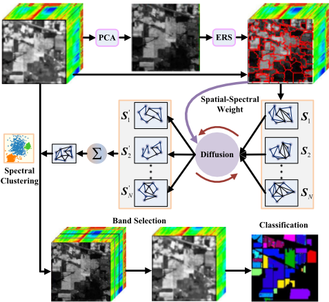
However, there are still at least two issues that hinder the band selection performance. Firstly, most of existing clustering based methods only take the correlation between neighbouring bands into account, while neglect the global information. Secondly, most of previous methods regard a certain band as a whole and reshape it to a feature vector, while the different reflection characteristics of objects are not exploited. In this paper, in order to tackle these two issues, we propose a hyperspectral band selection method via region-wise multiple graph fusion-based spectral clustering (RMGF). Since different objects are with different reflection characteristics, we first segment the first principal component of original hyperspectral image cube into homogeneous regions by using a certain superpixel segmentation, then we construct a similarity graph to reflect the similarity between band pairs corresponding to each region. For each region-wise graph, we design a diffusion process to update it to approximate the unified graph that reflects the global similarity between different bands. During the diffusion process, the spatial and spectral distribution of different superpixels are taken consideration, i.e., spatially adjacent superpixels should contribute more to each other. Finally, an optimal similarity graph is generated by using the multiple updated graphs and spectral clustering is performed to obtain different band partitions for band selection.
In a nutshell, the main contributions of this work are summarized as follows:
- As far as we know, this is the first work that proposes to fuse multiple graphs for clustering based hyperspectral band selection.
- Instead of treating a certain hyperspectral band as a whole to calculate the similarities between band pairs, we segment the hyperspectral band into homogeneous regions by considering that different objects are often with different reflection characteristics.
- We design a graph diffusion strategy to fuse multiple graphs for learning a consensus similarity graph that reflects the global relationship of all the hyperspectral bands. Extensive experiments are conducted to demonstrate the superiority of our proposed method when compared with other state-of-the-art hyperspectral band selection methods.
2 RelatedWork
In this section, we introduce some related clustering-based hyperspectral band selection methods which our proposed method belongs to.
For clustering-based methods, each band is treated as a data point and all of the bands are partitioned into several groups. Then, for each group, the most representative band is selected to form a new band subset. Based on the hierarchical clustering structure, Mart´Inez-Us ´OMartinez-Uso et al. [Mart´Inez-Us ´OMartinez-Uso et al., 2007] proposed to select informative bands by minimizing the intra-class variance as well as maximizing the inter-class variance. In [Wang et al., 2018], the dynamic programming is used for hyperspectral band partition. By estimating the band noise, the band with minimum noise in each group is selected as the representative band [Wang et al., 2019]. In order to determine the appropriate number of selected bands, the context information is utilized with a fast neighborhood grouping method for hyperspectral band partition in a coarse to fine manner [Wang et al., 2020a]. In [Yuan et al., 2015], a novel descriptor is designed to reveal the context of HSI and a dual clustering method which includes the contextual information is proposed for band clustering. [Li et al., 2019]. Based on the concept of shared nearest neighbor, the local density of each band and the information entropy are combined to select the optimal band subset.
Although great success has been achieved by previous clustering-based hyperspectral band selection methods, the global information as well as the spatial distribution of objects with different reflection characteristics are not well taken into consideration, which induces unsatisfactory results. Following we will introduce our proposed method to handle these issues in detail.
3 ProposedMethodology
In this section, the detailed process of our proposed RMGF will be elaborated step by step. In summary, RMGF consists of four main parts, i.e., homogeneous region segmentation, region-wise similarity graph construction, similarity graph diffusion and spectral-clustering based band selection, as shown in Figure 1.
3.1 Homogeneous Region Segmentation
In most of previous band selection methods, the spectral value of different pixels in a certain band are often stacked to form a single feature vector for band selection. However, it is well known that different objects are often with different reflection characteristics. Therefore, different homogeneous regions in hyperspectral images should be treated differently. In this work, we segment hyperspectral volume into several homogeneous regions with each region representing a certain object. Considering the promising performance in both efficacy and efficiency, we adopt the entropy rate superpixel segmentation (ESR) method [Liu et al., 2011] to generate multiple homogeneous regions. Of course, other segmentation algorithms can also be used. Given a hyperspectral cube with size H × W × B which consists of B bands, in order to capture the major information of hyperspectral as well as reduce the computational cost, we first obtain the first principal component (denoted as Hf ) of the hyperspectral images by using principal component analysis (PCA) [Wold et al., 1987]. Then, we can generate N superpixels by performing ESR on Hf as follows:
where Rp is the p-th superpixel.
3.2 Region-wise Similarity Graph Construction
Based on the segmentation result of, for each superpixel, we can obtain corresponding multiple superpixels from different band which share the same pixel locations as the one in Hf . Then we can calculate the similarity between each superpixel pair that represent the same homogeneous region across different bands. In such a manner, a B × B similarity graph which reflects the similarity of different bands in terms of each region can be obtained. Specifically, supposing that the feature vector represents the spectral values of the p-th superpixel in the i-th band and j-th band can be denoted as xip and xjp , respectively, then the p-th similarity graph can be calculated as follows:
where Nk(xjp ) denotes the set of k nearest neighbors of xjp and σ is the kernel width of the Gaussian kernel function. Note that other distance measuring functions or learning strategies can be also used in Eq. (2) for calculating the similarity values. However, they are not our focus in this work and we just use the Euclidean distance for its simplicity and efficiency.
3.3 Similarity Graph Diffusion
Since there may be inaccurate values in the similarity graphs as obtained by Eq. (2), while there are often multiple superpixels which represent the same or similar object classes. Therefore, we design a diffusion strategy to update the initial similarity graphs by exploiting the supplementary information implied in different graphs [Tang et al., 2020].
Given an initial M × M similarity graph S which indicates the similarities between M sample points, a more faithful similarity graph ¯S can be learned via diffusion process. As indicated by the manifold ranking model [Zhou et al., 2004; Bai et al., 2017], we can obtain the new similarity graph ¯S by solving the following optimization problem:
where µ > 0 is a regularization parameter. D is a diagonal degree matrix with its i-th diagonal elements Dii = ∑Mj=1 Sij . As can be seen fromEq. (3), it consists of two terms. The first term is the analogy to local and global consistency [Zhou et al., 2003] which regularizes that if data point i is similar to data point j and data point p is also similar to data point q on original similarity graph S, then the learned new similarities ¯Sip and ¯Sjq should also be similar. The second term can be regarded as a fitting term which regularizes that that a good learned similarity graph should not change too much from its initial status.
As derived in [Bai et al., 2017], Eq. (3) has a closed-form solution as follows:
where α = 1 1+µ . vec(·) is an operator which vectorizes an input matrix by stacking its columns one by one and the corresponding inverse operator is denoted as vec(·)-1 . A ∈ RM2×M2 is the Kronecker product of A, i.e., A ⊗ A with A = D- 12 SD- 12 .
Motivated by the previous works [Donoser and Bischof, 2013] that run in an iterative manner, the iteratively similarity propagation can be also formulated as follows:
where t represents the t-th iteration time.
Eq. (5) has a obvious drawback since it can only update a single similarity graph. In this work, we design a diffusion strategy to update the multiple graphs corresponding to multiple regions of hyperspectral images by fully exploiting the complementarity among different graphs.
In a certain band of the hyperspectral images, the superpixels with similar spectral values or closer spatial locations are more likely to represent the same objects. Therefore, during the diffusion process, the similarity graphs corresponding to superpixels which are with similar spectral values as well as closer spatial locations should contribute more to each other. With this point in mind, for the similarity graph of the p-th superpixel, we design the diffusion process to update Sp as follows:
where α is a parameter to balance the updated graph and its initial status. In our experiments, on order to emphasize the updated graph, we empirically set α = 0.7. ωpq denotes the weight that the q-th graph contributes to the p-th graph, which can be defined as follows:
where xp and xq denote the p-th and q-th feature vector of the corresponding superpixel in the the first principal component (i.e., Hf ) of the hyperspectral images as introduced in previous section. lp and lq denote the center pixel location of the p-th and q-th superpixel in Hf . σsv and σsl are two parameters that control the spectral sensitivity and spatial sensitivity of the element distribution, respectively. In Eq. (7), the first term measures the spectral similarity of two superpixels while the second term measures the spatial distance of two superpixels.
By using Eq. (6), the connection information in different graphs can be interchanged iteratively to achieve the final unified graph. On one hand, similarity values of different similarity graphs are propagated to each other by the iterative diffusion process. On the other hand, the information from original similarity graphs are partially preserved by the scalar parameter α. In addition, the spectral and spatial similarity of different superpixels are used to weight the diffusion process for better exploiting the complementarity among multiple graphs.
After T times of diffusion, each single similarity graph corresponding to a superpixel can be updated to a stable status. Then the final unified graph which reflects the similarity of different hyperspectral bands can be obtained as follows:
which is used for final spectral clustering to partition original hyperspectral bands into several band subsets.
3.4 Spectral-clustering Based Band Selection
Given a certain number of bands K that we want to select, original hyperspectral bands can be partitioned to K subsets by performing spectral clustering algorithm on S∗ . As to each band subset, the band which is closest to the subset center is selected as the representative band.
3.5 Theoretical Analysis of the Diffusion Process
Computational Complexity Analysis
As can be seen from Eq. (6), after we obtain the initial similarity graphs of different superpixels, the major computational cost of each diffusion iteration is the multiplication operation of matrices with size B ×B, of which the computational time complexity is O(B3 ). Therefore, the whole computational time complexity of the diffusion process is O(TB3 ), where T is the final iteration times.
Theoretical Convergence Analysis
In this section, we give the theoretical convergence analysis of the iterative diffusion process. Similar to [Bai et al., 2017], we firstly introduce the following Lemma 1.
Lemma 1. Given three matrices X, Y and Z with appropriate sizes, then vec(XYZT ) = (Z ⊗ X)vec(Y).
By applying vec(·) to both sides of Eq. (6), we have
Since the spectral radius of A is no larger than 1, according to the properties of Kronecker product, the eigenvalues of A = A ⊗ A are also in [-1, 1]. Since 0 < α < 1, we have
Therefore, when t →∞, Eq. (9) converges as
By applying vec-1 to both sides of Eq. (11), the iteration converges to exactly the same solution in Eq. (4).
4 Experiments
In this section, extensive experiments are conducted on three commonly used public hyperspectral image datasets to demonstrate the efficacy of the proposed method.
4.1 Datasets
Three datasets include Indian Pines scene, Pavia University Scene and Salinas Scene are used for our experiments. The detailed information are as follows.
Indian Pines Scene: This dataset was collected by the AVIRIS sensor in 1992, which consists of 224 spectral bands with the size of 145 × 145 pixels from 0.4 to 2.5µm. There are 16 different classes of land cover objects in the scene. Since some bands (104-108, 150-163, and 220) are with heavy noises due to water absorption, we discard those noisy bands and finally fetch 200 bands for experiments.
Pavia University Scene: This dataset was captured over Pavia by the ROSIS sensor in 2002. Similar to the Indian Pines dataset, after removing some noisy bands, 103 spectral bands are remained. The size of each band is 610 and there are 9 classes of land cover objects in this scene.
Salinas Scene: This dataset was also gathered by the AVIRIS sensor over Salinas Valley, CA, USA, in 1998. This dataset is with a high spatial resolution (3.7-m pixels) and has a total of 224 spectral bands with the size of 512 × 217. There are 16 classes of land cover objects in this scene.
| Datasets | Classifiers | UBS | TOF | ASPS MN | ASPS IE | FNGBS | ONR | RMGF |
|---|---|---|---|---|---|---|---|---|
| Indian Pines | KNN | 66.40±0.17 | 68.55±0.14 | 70.92±0.12 | 71.34± 0.12 | 71.48±0.14 | 69.98±0.26 | 76.26±0.16 |
| SVM | 80.09±0.16 | 79.48±0.17 | 81.20±0.25 | 81.26± 0.16 | 81.77±0.17 | 80.25±0.37 | 86.48±0.17 | |
| LDA | 71.12±0.18 | 70.90±0.10 | 70.46±0.32 | 70.20± 0.22 | 70.52±0.16 | 70.09±0.20 | 81.19±0.12 | |
| Pavia University | KNN | 86.43±0.07 | 86.00±0.04 | 87.28±0.15 | 87.07±0.06 | 87.36±0.05 | 89.10±0.15 | 91.76±0.13 |
| SVM | 94.33±0.05 | 94.10±0.02 | 94.08±0.26 | 93.95± 0.14 | 94.46±0.07 | 94.27±0.14 | 96.35±0.09 | |
| LDA | 84.19±0.06 | 84.16±0.08 | 84.06±0.16 | 83.62±0.09 | 84.20±0.04 | 83.48±0.13 | 90.49±0.07 | |
| Salinas | KNN | 89.33±0.03 | 88.95±0.05 | 89.38±0.14 | 89.14±0.04 | 89.24±0.05 | 89.33± 0.13 | 92.35±0.12 |
| SVM | 93.26±0.04 | 93.46±0.04 | 93.13±0.15 | 93.08± 0.05 | 93.25±0.06 | 93.35±0.16 | 95.00±0.11 | |
| LDA | 90.41±0.04 | 90.31±0.03 | 90.30±0.06 | 89.93±0.02 | 90.37±0.03 | 90.69±0.15 | 92.32±0.08 |
4.2 ComparedMethods
In order to validate the superiority of our proposed RMGF, five other unsupervised hyperspectral band selection methods are used for comparison, they are as follows:
- UBS [Chang and Wang, 2006], which divides the hyperspectral image cube into multiple subcubes at equal width based on the required number of selected bands, each segmentation point is viewed as the representative band.
- TOF [Wang et al., 2018], which aims to construct an optimal clustering model with rank constraint to provide an effective criterion for selecting bands on existing clustering structure.
- ASPS MN [Wang et al., 2019], which performs hyperspectral band selection via an adaptive subspace partition strategy. The representative band of each band subset is selected based on band noise estimation.
- ASPS IE [Wang et al., 2019], similar to ASPS MN that selects representative bands from band subsets, but it differs to ASPS MN that the representative band of each band subset is selected by the information entropy.
- FNGBS [Wang et al., 2020a], which is a fast neighborhood grouping method for hyperspectral band selection. The band with the highest local density and information entropy of each band subset is selected.
- ONR [Wang et al., 2020b], which selects those bands that are with high capability to reconstruct other bands and formulates the band selection as a combinatorial optimization problem.
4.3 Experimental Setup
In our experiments, three typical classifiers, including k-nearest neighborhood (KNN), support vector machine (SVM), and linear discriminant analysis (LDA), are used to evaluate the classification performance of different band selection algorithms. Since the desired number of selected bands is unknown and yet difficult to determine in practice for different datasets, we vary the number of selected bands from 5 to 60 with step 5 to illustrate the influence of different numbers of bands on the final classification accuracy. The parameter k of KNN is set to 3 for all experiments. For the SVM classifier, we implement it with the RBF kernel, and the penalty C and gamma are set 1e4 and 0.5, respectively.
For each dataset, 10% samples of each class are randomly chosen to construct the training set, and the rest 90% samples are used for testing. In addition, we perform each algorithm ten times and report the average results for reducing the influence of random selection of training and testing samples.
4.4 Experimental Results
In order to validate the efficacy of the proposed method, we compare it with other six state-of-the-art ones by using three different classifiers. By selecting the optimal number of selected bands, the overall accuracy (OA) of different methods on three different datasets are shown in Table 1. The best results are highlighted in bold font. As can be seen, our proposed RMGF consistently outperforms other competitors in terms of different classifiers on all of the three datasets.
As to the Indian Pines dataset, our RMGF obtains more than 7% OA when compared to other methods by using different classifiers. Specially, when using LDA as classifier, RMGF gains more than 10% OA. For Pavia University dataset, when using LDA as classifier, RMGF also obtains more than 5% improvement than other methods.
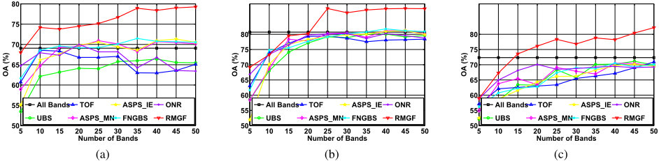
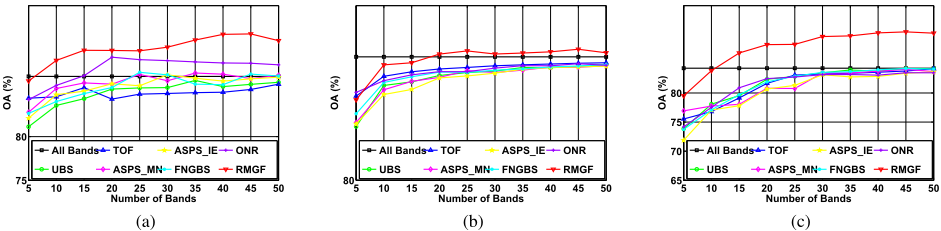
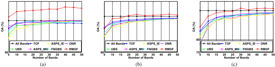
As aforementioned, it is difficult to determine the desired number of selected bands in practice for different datasets, we plot the OA curves for every five bands for each dataset in Figure 2-4. As can be seen, our proposed method outperforms other ones in most of the numbers of selected bands. As shown in Figure 2 and 3, by performing KNN and LDA on the selected bands of RMGF, we can always obtain higher OA on Indian Pines and Pavia University datasets. In Figure 4, we can see that RMGF can always select more discriminative bands for different classifiers.
5 Conclusion
In this paper, we present a hyperspectral band selection method via spatial-spectral weighted region-wise multiple graph fusion-based spectral clustering (RMGF). By considering that different objects have different reflection characteristics, we partition the hyperspectral images into multiple homogeneous regions, with each region representing the same class of object. For each region across different bands, we constructs a corresponding similarity graph to reflect the similarity between band pairs. Then, a spatial-spectral weighted multiple graph fusion strategy is designed to learn a unified graph for final band clustering. The optimal bands are selected based on the clustering results. Extensive experiments on three datasets are conducted to demonstrate the superiority of RMGF when compared with other state-of-the-art methods.
Acknowledgements
The work was supported in part by the National Science Foundation (NSF) of China (No. 62076228); in part by National Key R&D Program of China (No. 2020AAA0107100); in part by Natural Natural Science Foundation of Hubei Province (No. 2020CFB644); in part by the Opening Fund of Key Laboratory of Geological Survey and Evaluation of Ministry of Education (No. GLAB2020ZR18) and the Fundamental Research Funds for the Central Universities; Sponsored by CAAI-Huawei MindSpore Open Fund, see [Huawei Technologies Co., 2020].
@inproceedings{ijcai2021p418,
  title     = {Hyperspectral Band Selection via Spatial-Spectral Weighted Region-wise Multiple Graph Fusion-Based Spectral Clustering},
  author    = {Tang, Chang and Liu, Xinwang and Zhu, En and Wang, Lizhe and Zomaya, Albert},
  booktitle = {Proceedings of the Thirtieth International Joint Conference on
               Artificial Intelligence, {IJCAI-21}},
  publisher = {International Joint Conferences on Artificial Intelligence Organization},
  editor    = {Zhi-Hua Zhou},
  pages     = {3038--3044},
  year      = {2021},
  month     = {8},
  note      = {Main Track},
  doi       = {10.24963/ijcai.2021/418},
  url       = {https://doi.org/10.24963/ijcai.2021/418},
}
TY - CPAPER TI - Hyperspectral Band Selection via Spatial-Spectral Weighted Region-wise Multiple Graph Fusion-Based Spectral Clustering AU - Tang, Chang AU - Liu, Xinwang AU - Zhu, En AU - Wang, Lizhe AU - Zomaya, Albert T2 - Proceedings of the Thirtieth International Joint Conference on Artificial Intelligence, IJCAI-21 PB - International Joint Conferences on Artificial Intelligence Organization PY - 2021 SP - 3038 EP - 3044 DO - 10.24963/ijcai.2021/418 UR - https://doi.org/10.24963/ijcai.2021/418 ER -Copied
Machine-readable versions of this paper, for tools and AI agents:





