
Regularizing Variational Autoencoder with Diversity and Uncertainty Awareness
Proceedings of the Thirtieth International Joint Conference on Artificial Intelligence. Main Track. Pages 2964-2970.
https://doi.org/10.24963/ijcai.2021/408
Keywords
- Machine Learning: Probabilistic Machine Learning
- Machine Learning: Unsupervised Learning
- Machine Learning: Bayesian Learning
Abstract
As one of the most popular generative models, Variational Autoencoder (VAE) approximates the posterior of latent variables based on amortized variational inference. However, when the decoder network is sufficiently expressive, VAE may lead to posterior collapse; that is, uninformative latent representations may be learned. To this end, in this paper, we propose an alternative model, DU-VAE, for learning a more Diverse and less Uncertain latent space, and thus the representation can be learned in a meaningful and compact manner. Specifically, we first theoretically demonstrate that it will result in better latent space with high diversity and low uncertainty awareness by controlling the distribution of posterior’s parameters across the whole data accordingly. Then, without the introduction of new loss terms or modifying training strategies, we propose to exploit Dropout on the variances and Batch-Normalization on the means simultaneously to regularize their distributions implicitly. Furthermore, to evaluate the generalization effect, we also exploit DU-VAE for inverse autoregressive flow based-VAE (VAE-IAF) empirically. Finally, extensive experiments on three benchmark datasets clearly show that our approach can outperform state-of-the-art baselines on both likelihood estimation and underlying classification tasks.
- [Alemi et al., 2016] Alexander A Alemi, Ian Fischer, Joshua V Dillon, and Kevin Murphy. Deep variational information bottleneck. ICLR, 2016.
- [Bowman et al., 2015a] Samuel R Bowman, Gabor Angeli, Christopher Potts, and Christopher D Manning. A large annotated corpus for learning natural language inference. In EMNLP, 2015.
- [Bowman et al., 2015b] Samuel R Bowman, Luke Vilnis, Oriol Vinyals, Andrew M Dai, Rafal Jozefowicz, and Samy Bengio. Generating sentences from a continuous space. CCNLP, 2015.
- [Burda et al., 2016] Yuri Burda, Roger B Grosse, and Rus- lan Salakhutdinov. Importance weighted autoencoders. In ICLR, 2016.
- [Chen et al., 2017] Xi Chen, Diederik P. Kingma, Tim Sal- imans, Yan Duan, P. Dhariwal, John Schulman, Ilya Sutskever, and P. Abbeel. Variational lossy autoencoder. ICLR, 2017.
- [Fang et al., 2019] Le Fang, Chunyuan Li, Jianfeng Gao, Wen Dong, and Changyou Chen. Implicit deep latent vari- able models for text generation. In EMNLP, 2019.
- [Fu et al., 2019] Hao Fu, Chunyuan Li, Xiaodong Liu, Jian- feng Gao, Asli Celikyilmaz, and Lawrence Carin. Cycli- cal annealing schedule: A simple approach to mitigating kl vanishing. In ACL, 2019.
- [He et al., 2016] Kaiming He, Xiangyu Zhang, Shaoqing Ren, and Jian Sun. Deep residual learning for image recog- nition. In CVPR, 2016.
- [He et al., 2018] Junxian He, Daniel Spokoyny, Graham Neubig, and Taylor Berg-Kirkpatrick. Lagging infer- ence networks and posterior collapse in variational autoen- coders. In ICLR, 2018.
- [Higgins et al., 2017] I. Higgins, Loïc Matthey, A. Pal, C. Burgess, Xavier Glorot, M. Botvinick, S. Mohamed, and Alexander Lerchner. beta-vae: Learning basic vi- sual concepts with a constrained variational framework. In ICLR, 2017.
- [Hochreiter and Schmidhuber, 1997] Sepp Hochreiter and Jürgen Schmidhuber. Long short-term memory. Neural computation, 9(8):1735-1780, 1997.
- [Ioffe and Szegedy, 2015] Sergey Ioffe and Christian Szegedy. Batch normalization: Accelerating deep net- work training by reducing internal covariate shift. ICML, 2015.
- [Kim et al., 2018] Yoon Kim, Sam Wiseman, Andrew Miller, David Sontag, and Alexander Rush. Semi- amortized variational autoencoders. In ICML, 2018.
- [Kingma and Ba, 2015] Diederik P Kingma and Jimmy Ba. Adam: A method for stochastic optimization. ICLR, 2015.
- [Kingma and Welling, 2013] Diederik P Kingma and Max Welling. Auto-encoding variational bayes. ICLR, 2013.
- [Kingma et al., 2016] Durk P Kingma, Tim Salimans, Rafal Jozefowicz, Xi Chen, Ilya Sutskever, and Max Welling. Improved variational inference with inverse autoregressive flow. In NeurIPS, 2016.
- [Lake et al., 2015] Brenden M Lake, Ruslan Salakhutdinov, and Joshua B Tenenbaum. Human-level concept learn- ing through probabilistic program induction. Science, 350(6266):1332-1338, 2015.
- [Ma et al., 2018] Xuezhe Ma, Chunting Zhou, and Eduard Hovy. Mae: Mutual posterior-divergence regularization for variational autoencoders. In ICLR, 2018.
- [Makhzani et al., 2016] Alireza Makhzani, Jonathon Shlens, Navdeep Jaitly, and Ian J. Goodfellow. Adversarial au- toencoders. ICLR, 2016.
- [Pu et al., 2016] Yunchen Pu, Zhe Gan, Ricardo Henao, Xin Yuan, Chunyuan Li, Andrew Stevens, and Lawrence Carin. Variational autoencoder for deep learning of im- ages, labels and captions. In NeurIPS, 2016.
- [Razavi et al., 2018] Ali Razavi, Aaron van den Oord, Ben Poole, and Oriol Vinyals. Preventing posterior collapse with delta-vaes. In ICLR, 2018.
- [Shen et al., 2017] Tianxiao Shen, Tao Lei, Regina Barzilay, and Tommi Jaakkola. Style transfer from non-parallel text by cross-alignment. In NeurIPS, 2017.
- [Srivastava et al., 2014] Nitish Srivastava, Geoffrey Hinton, Alex Krizhevsky, Ilya Sutskever, and Ruslan Salakhutdi- nov. Dropout: a simple way to prevent neural networks from overfitting. JLMR, 15(1):1929-1958, 2014.
- [Van den Oord et al., 2016] Aaron Van den Oord, Nal Kalchbrenner, Lasse Espeholt, Oriol Vinyals, Alex Graves, et al. Conditional image generation with pixelcnn decoders. In NeurIPS, pages 4790-4798, 2016.
- [Yang et al., 2017] Zichao Yang, Zhiting Hu, Ruslan Salakhutdinov, and Taylor Berg-Kirkpatrick. Improved variational autoencoders for text modeling using dilated convolutions. In ICML, 2017.
- [Zhao et al., 2019] Shengjia Zhao, Jiaming Song, and S. Er- mon. Infovae: Balancing learning and inference in varia- tional autoencoders. In AAAI, 2019.
- [Zheng et al., 2019] Huangjie Zheng, Jiangchao Yao, Ya Zhang, Ivor W Tsang, and Jia Wang. Understanding vaes in fisher-shannon plane. In AAAI, 2019.
- [Zhu et al., 2020] Qile Zhu, Wei Bi, Xiaojiang Liu, Xiyao Ma, Xiaolin Li, and D. Wu. A batch normalized inference network keeps the kl vanishing away. In ACL, 2020.
References were extracted automatically from the PDF and may contain errors.
Full text extracted automatically from the PDF; figures, tables and equations may differ. The PDF is the version of record.
1 Introduction
Recent years have witnessed the great success of Variational Autoencoder (VAE) [Kingma and Welling, 2013] as a generative model for representation learning, which has been widely exploited in various challenging domains, such as natural language modeling and image processing [Bowman et al., 2015b; Pu et al., 2016]. Indeed, VAE models the generative process of observed data by defining a joint distribution with latent space, and approximates the posterior of latent variables based on the amortized variational inference. While the use of VAE has been well-recognized, it may lead to uninformative latent representations, particularly when the expressive and powerful decoder networks are employed, such as LSTMs [Hochreiter and Schmidhuber, 1997] on text or PixelCNN [Van den Oord et al., 2016] on images. This is widely known as the posterior collapse phenomenon [Zhao et al., 2019]. In other words, the model may fail to diversify the posteriors of different data by simply using the single posterior distribution component to model all data instances. Also, the traditional VAE model usually produces the redundant information of representation due to the lack of guidance to characterize posterior space [Bowman et al., 2015a; Chen et al., 2017]. Therefore, the learned representation of VAE often results in an unsatisfied performance for downstream tasks, such as classification, even if it can approximate the marginal likelihood of observed data very well.
∗This work was done when Dazhong Shen was an intern at Talent Intelligent Center, Baidu Inc. Hui Xiong and Hengshu Zhu are the corresponding authors.
In the literature, tremendous efforts have been made for improving the representation learning of VAE and alleviating the problem of posterior collapse. One thread of these works is to attribute the posterior collapse to optimization challenges of VAEs and design various strategies, including KL annealing [Bowman et al., 2015a; Fu et al., 2019], FreeBits(FB) [Kingma et al., 2016], aggressive training [He et al., 2018], encoder network pretraining and decoder network weakening [Yang et al., 2017]. Among them, BN-VAE [Zhu et al., 2020] applies the Batch-Normalization (BN) [Ioffe and Szegedy, 2015] to ensure one positive lower bound of the KL term. However, the theoretical basis of the effectiveness of BN on latent space learning is not yet understood, and more possible explanations based on the geometry analysis of latent space are needed. Other studies attempt to modify the objective carefully to direct the latent space learning [Makhzani et al., 2016; Zheng et al., 2019]. One feasible direction is to add additional Mutual Information (MI) based term to enhance the relation between data and latent space. However, due to the intractability, additional designs are always required for approximating MI-based objectives [Fang et al., 2019; Zhao et al., 2019]. Recently, Mutual Posterior-Divergence (MPD) [Ma et al., 2018] is introduced to measure the diversity of the latent space, which is analytic and has one similar goal with MI. However, the scales of MPD and original objective are unbalanced, which requires deliberate normalization.
In this paper, to improve the representation learning performances of VAE, we propose a novel generative model, DU- VAE, for learning a more Diverse and less Uncertain latent space, and thus ensures the representation can be learned in a meaningful and compact manner. To be specific, we first analyze the expected latent space theoretically from two geometry properties, diversity and uncertainty, based on the MPD and Conditional Entropy (CE) metrics, respectively. We demonstrate that it will lead to a better latent space with high diversity and low uncertainty by controlling the distribution of posterior's parameters across the whole data. Then, instead of introducing new loss terms or modifying training strategies, we propose to apply Dropout [Srivastava et al., 2014] on the variances and Batch-Normalization on the means simultaneously to regularize their distributions implicitly. In particular, we also discuss and prove the effectiveness of two regularizations in a rigorous way. Furthermore, to verify the generalization of our approaches, we also demonstrate that DU-VAE can be extended empirically into VAEIAF [Kingma et al., 2016], a well-known normalizing flowbased VAE. Finally, extensive experiments have been conducted on three benchmark datasets, and the results clearly show that our approach can outperform state-of-the-art baselines on both likelihood estimation and classification tasks.
2 Background of VAE
Given the input space x ∈ X , VAE aims to construct a smooth latent space z ∈ Z by learning a generative model p(x, z). Starting from a prior distribution p(z), such as standard multivariate Gaussian N(0, I), VAE generates data with a complex conditional distribution pθ(x|z) parameterized by one neural network fθ(·). The goal of the model training is to maximize the marginal likelihood EpD(x)[log pθ(x)], where the pD(x) is the true underlying distribution. To calculate this intractable marginal likelihood, an amortized inference distribution qφ(z|x) parameterized by one neural network fφ(·) has been utilized to approximate the true posterior. Then, it turns out to optimize the following lower bound:
where the first term is the reconstruction loss and the second one is the Kullback-Leibler (KL) divergence between the approximated posterior and prior.
Unfortunately, in practice, VAE may fail to capture meaningful representation. In particular, when applying autoregressive models as the decoder network, such as LSTMs or PixelCNN, it is likely to model the data marginal distribution pD(x) very well even without latent variable z, i.e., p(x|z) = Πip(xi|x<i). In this case, VAE degenerates to auto-regressive, the latent variable z tends to be independent with the data x. Meanwhile, with the goal to minimize DKL[q(z|x)||p(z)] in ELBO objective, q(z|x) vanishes to p(z), i.e., q(z|xi) = q(z|xj) = p(z), ∀xi, xj ∈ X. To solve this problem, we will direct the latent space learning carefully and purposefully for high diversity and low uncertainty in the following.
3 The ProposedMethod
Here, we start with theoretical analysis on the latent space of VAE from two geometric properties: diversity and uncertainty, respectively. Then, we design Dropout on the variance parameters and Batch-Normalization on the mean parameters to encourage the latent space with high diversity and low uncertainty. In particular, the effectiveness of our approach will be discussed and proved rigorously. Finally, we extend DUVAE into VAE-IAF [Kingma et al., 2016] empirically.
3.1 Geometric Properties of Latent Space
For enabling meaningful and compact representation learning in VAE model, we have two intuitions: 1) for different data samples x1, x2, the posteriors q(z1|x1) and q(z2|x2) should mutually diversify from each other, which encourages posteriors to capture the characteristic or discriminative information from data; 2) given data sample x, the degree of uncertainty of the latent variable z should be minimized, which encourages removing redundant information from z. Guided by those intuitions, we first analyze the diversity and uncertainty of latent space under quantitative metric, respectively.
Diversity of Latent Space
Here, we attempt to measure the divergence among the posterior distribution family. One intuitive and reasonable metric is the expectation of the mutual divergence between a pair of posteriors. Following this idea, [Ma et al., 2018] proposed the mutual posterior diversity (MPD) to measure the diversity of posteriors, which can be computed by:
where x1, x2 ∼ pD(x) are i.i.d. and DSKL[q1||q2] is symmetric KL divergence defined as the mean of DKL[q2||q1] and DKL[q2||q1], which is analytical under Gaussian distributions. Specifically, we have:
Interestingly, if the value of δ2x,d is upper bounded, like less than 1 in most practical case for VAEs. then, we can find that MPD has one lower and strict bound proportional to ∑nd=1 V arPD(x) [µx,d] (see Supplementary).
Uncertainty of Latent Space
Here, we aim at quantifying the uncertainty about the outcome of latent variable z given data sample x and the learned encoder distribution qφ(z|x). In information theory, conditional entropy is utilized to measure the average level of the uncertainty inherent in the variable's possible outcomes when giving another variable. Due to the same goal, we follow this idea and use the Conditional Entropy (CE) Hqφ (z|x) for z conditioned on x to measure the uncertainty of latent space:
where H(qφ(z|x)) denotes the differential entropy of posterior qφ(z|x). Actually, H(qφ(z|x)) can be computed analytically as ∑nd=1 1 2 log(2πeδ2x,d ), then we have:
Intuitively, in order to reduce the uncertainty in the latent space, we need to minimize the conditional entropy Hqφ (z|x). However, the differential entropies H(qφ(z|x)) defined on continuous spaces are not bounded from below. That is, the variance δ2x,d can be scaled to be arbitrarily small achieving arbitrarily high-magnitude negative entropy. As a result, the optimization trajectories will invariably end with garbage networks as activations approach zero or infinite. To solve this problem, we enforce the differential entropy nonnegativity by adding noise to the latent variable. For one latent variable z, we replace it with z + ϵ, where ϵ ∼ N(0, α) is one zero-entropy noise, where we set constant α = 1 2πe for convenience. Then based on properties of Gaussian distribution, we have H(qφ(z|x)) > H(ϵ) = 0 and δ2x,d > α.
In sum, in order to encourage the diversity and decrease the uncertainty of latent space, we need to constrain both MPD in Equation 3 and CE in Equation 4 . One feasible solution is to regard them as additional objectives explicitly and approximate them by using Monte Carlo in each mini-batch. However, the scales among different objective terms are unbalanced, which require deliberately designed normalization or careful weight parameters tuning [Ma et al., 2018].
Instead, we propose control implicitly the MPD and CE without modifying the objective function. Based on Equation 3 and Equation 4, we note that both MPD and CE are only dependent on approximated posterior' s parameters, i.e., µx,d or δx,d. This inspires us to select proper regularization on the distribution of posterior' s parameters to encourage higher MPD and lower CE. Specifically, in the following two sub-sections. we will introduce the application of the Dropout on variance parameters and Batch-Normalization on mean parameters respectively, and provide theoretical analysis about the effectiveness of our approach.
3.2 Dropout on Variance Parameters
In order to encourage high diversity and low uncertainty of latent space, we need to increase the MPD in Equation 3 and decrease the CE in Equation 5, simultaneously. Meanwhile, we also need to avoid EpD(x)[δ2x,d ] to be too small for ensuring the smoothing of the latent space. One extreme case is that when EpD(x)[δ2x,d ] convergence to 0, i.e., δ2x,d ≈ 0, ∀x, d, each data point is associated with a delta distribution in latent space and the VAEs degenerate into Autoencoders in this dimension. To accomplish these requirements together, we propose to apply Dropout [Srivastava et al., 2014] to regularize posterior's variance parameters in training as following,
where gx,d denotes the independent random variable generated from the normalized Bernoulli distribution 1/pB(1, p), p ∈ (0, 1), where EB[gx,d] = 1. Then, we have the following proposition (see Supplementary for the proof.):
Proposition 1. Given the Dropout strategy defined in Equation 6, we have:
Algorithm 1 Training Procedure of DU-VAE
- 1: Initialize φ, θ, γµ = γ, and βµ = 0
- 2: while not convergence do
- 3: Sample a mini-batch x
- 4: µx, δ2x = fφ(x).
- 5: ˆµx = BNγµ,βµ (µx), ˆ δ2x = Dropoutp(δ2x ).
- 6: Sample z ∼N(ˆµx, ˆ δ2x ) and generate x from fθ(z).
- 7: Compute gradients gφ,θ ←∇φ,θLELBO(x; φ, θ).
- 8: Update φ, θ, γµ, βµ according to gφ,θ.
- 9: γµ = γ √E[γ 2µ ] ⊙ γµ
- 10: end while
where two inequalities are both strict, the gaps between two sides are greater as p decreases to 0. Then, we also have:
Proposition 1 tells us that: 1) Dropout regularization encourages the increase of MPDpD(x)[z] and the decrease of the conditional entropy Hqφ (z|x) of the latent space while preserving the expectation of variance parameters, which is actually a simple but useful strategy what we need. 2) Dropout regularization also provides one lower bound of MPDpD(x)[z] independent on the variance parameters, which makes it possible to ensure positive MPD with further controls on the variance ∑nd=1 V arpD(x)[µx,d].
3.3 Batch-Normalization onMean Parameters
Inspired by Batch-Normalization (BN) [Ioffe and Szegedy, 2015], which is an effective approach to control the distribution of the output of neural network layer. We apply BN on the mean parameters µx,d to constrain ∑nd=1 V arpD(x)[µx,d]. Mathematically, our BN is defined as:
where ˆµx,d represents the output of BN layer, and µBd and δBd denote the mean and standard deviation of µx,d estimated within each mini-batch. γµd and βµd are the scale and shift parameters, which lead that the distribution of ˆµx,d has the variance γ 2µd and mean βµd . Therefore, we can control the ∑nd=1 V arpD(x)[µx,d] by fixing the mean Ed[γ 2µd ] = γ 2 with respect to each dimension d. Specifically, we regard each γd as learnable parameters with initialization γ. Then after each training iteration, we re-scale each parameter γµd with coefficient γ/√Ed[γ 2µd ]. In addition, all βµd is learnable with initialization 0 and no constraint.
Overall, based on the analysis above, we propose our approach, namely DU-VAE, to encourage high diversity and low uncertainty of the latent space by applying Dropout regularizations on variance parameters and Batch-Normalization on mean parameters of approximated posteriors, simultaneously. Specifically, we train DU-VAE following Algorithm 1. Connections with BN-VAE. In the literature, BN-VAE [Zhu et al., 2020] also applies BN on mean parameters. Zhu et al. claim that keeping one positive lower bound of the KL term, i.e., the expectation of the square of mean parameters ∑nd=1 Eqφ [µ2x,d ], is sufficient for preventing posterior collapse. In practice, they ensure Eqφ [µ2x,d ] > 0 by fixing scale parameter γµd of BN for each dimension d. However, here, we will demonstrate that keeping one positive lower bound of MPD is one more powerful strategy for preventing collapse posterior. As the discussion in Section 2, when posterior collapse occurs, we have q(z|xi) = q(z|xj) = p(z), ∀xi, xj ∈ X. Therefore, to avoid this phenomenon, we actually need to control posterior distributions carefully so that:
where the first term is actually implied in the second term as the necessary condition and DKL[q(z|x)||p(x)] > 0 is equivalent (both sufficient and necessary) to the first term, we can claim that keeping one positive lower bound of the KL term is not sufficient for the second term along with several certain abnormal cases (detailed analysis can be found in Supplementary.). By contrast, keeping one positive MPD in the latent space is actually one equivalent condition for the second term, which implies the first term. Actually, from the perspective of the diversity of latent space, we can provide one more possible explanation for the effectiveness of BNVAE. That is, the application of BN on µx ensures one positive value of V arpD(x)[µx, d] for each d, which is also one lower bound of MPD defined in Equation 2 when the variance parameters has one constant upper bound, like 1 in practice.
3.4 Extension to VAE-IAF
Here, to further examine the generalization of DU-VAE, we aim to extend our approach for other VAE variants, such as, VAE-IAF [Kingma et al., 2016], one well-known normalizing flow-based VAE. Different from classic VAEs which assume the posterior distributions are diagonal Gaussian distributions, VAE-IAF can construct more flexible posterior distributions through applying one chain of invertible transformations, named the IAF chain, on an initial random variable drown from one diagonal Gaussian distribution. Specifically, the initial random variable z0 is sampled from the diagonal Gaussian with parameters µ0 and δ0 outputted from the encoder network. Then, T invertible transformations, are applied to transform z0 into the final random variable zT . More details can be found in [Kingma et al., 2016].
Indeed, noting that the MPD and CE of the initial random variable z0 have the same form as these for classic VAEs in Equation 2 and Equation 4, one intuitive idea is to apply Dropout on δ0 and Batch Normalization on µ0 with the guidance in Algorithm 1 to control the MPD and CE of z0 . It is surprising to find that this simple extension of DU-VAE, called DU-IAF, demonstrated comparative performance in our experiments. This may be attributed to the close connection between z0 and zT . In particular, we find that the CE of z0 is the upper bound of CE of zT . Meanwhile, MPDpD(x)[z0 ] is closely related with MPDpD(x)[zT ], even they are equal to each other when each invertible transformation in IAF chain is independent on the input data. Further discussion and proof can be found in Supplementary.
4 Experiments
In this section, our method would be evaluated on three benchmark datasets in terms of various metrics and tasks. Complete experimental setup can be found in Supplementary.
4.1 Experimental Setup
Setting. Following the same configuration as [He et al., 2018], we evaluated our method on two text benchmark datasets, i.e., Yahoo and Yelp corpora [Yang et al., 2017] and one image benchmark dataset, i.e., OMNIGLOT [Lake et al., 2015]. For text datasets, we utilized a single layer LSTM as both encoder and decoder networks, where the initial state of the decoder is projected by the latent variable z. For images, a 3-layer ResNet [He et al., 2016] encoder and a 13-layer Gated PixelCNN [Van den Oord et al., 2016] decoder are applied. We set the dimension of z as 32. and utilized SGD to optimize the ELBO objective for text and Adam [Kingma and Ba, 2015] for images. Following [Burda et al., 2016], we utilized dynamically binarized images for training and the fixed binarization as test data. Meanwhile, following [Bowman et al., 2015a], we applied a linear annealing strategy to increasing the KL weight from 0 to 1 in the first 10 epochs if possible. Evaluation Metrics. Following [Burda et al., 2016], we computed the approximate negative log-likelihood (NLL) by estimating 500 importance weighted samples. In addition, we also considered the value of KL term, mutual information (MI) I(x, z) [Alemi et al., 2016] under the joint distribution q(x, z) and the number of activate units (AU) [He et al., 2018] as additional metrics. In particular, the activity of each dimension zd is measured as Az,d = Cov(Ezd∼q(zd|x)[zd]). One dimension is regarded to be active when Az,d > 0.01. Baselines. We compare our method with various VAE-based models, which can be grouped into two categories: 1) Classic VAEs: VAE with annealing [Bowman et al., 2015a]; SemiAmortized VAE (SA-VAE) [Kim et al., 2018]; Agg-VAE [He et al., 2018]; β-VAE [Higgins et al., 2017] with parameter β re-weighting the KL term; FB [Kingma et al., 2016] with parameter λ constraining the minimum of KL term in each dimension; δ-VAE [Razavi et al., 2018] with parameter δ constraining the range of KL term; BN-VAE [Zhu et al., 2020] with parameter γ keeping one positive KL term; MAE [Ma et al., 2018] with parameters γ and η controlling the diversity and smoothness of the latent space. Note that we implemented MAE with the standard Gaussian prior, instead of the AF prior in [Ma et al., 2018] for one fair comparison. 2) IAF-based models: IAF+FB [Kingma et al., 2016], which utilized the FB strategy with the parameter λ to avoid the posterior collapse in VAE-IAF; IAF+BN, where we applied BN regularization on the mean parameters of the distributions of z0 with the fixed scale parameters γ in each dimension.
4.2 Overall Performance
Log-Likelihood Estimation. Table 1 shows the results in terms of log-likelihood estimation. We can note that DUVAE and DU-IAF achieve the best NLL among classic VAEs and IAF-based VAEs in all datasets, respectively. Besides, we also have some interesting findings. First, MAE does not perform well in all datasets, which may be caused by the difficulty to balance the additional training objective terms and ELBO. Second, although, Agg-VAE and SA-VAE also reach the great NLL in both datasets, they require the additional training procedure on the inference network, leading to the high training time cost [Zhu et al., 2020]. Third, BNVAE also achieves completive performance on text datasets. However, for images, where the posterior collapse may be less of an issue [Kim et al., 2018], BN-VAE fails to catch up with other models, even worse than basic VAE on NLL. Fourth, DU-VAE prefers to capture higher KL and MI compared with BN-VAE with the same scale parameter γ. In other words, DU-VAE can convert more information from the observed data into the latent variable. Fifth, based on the results of IAF+BN, we can find that the BN strategy used in BN-VAE can not prevent the collapse posterior in VAE-IAF with small KL. By contrast, our approach can be easily extended for VAE-IAF with the best performance. Finally, we also note that IAF based models may be more suitable for image dataset without sound performance on text, while DUIAF nevertheless achieves competitive performance.
| Yahoo | Yelp | OMNIGLOT | ||||||||||
|---|---|---|---|---|---|---|---|---|---|---|---|---|
| Model | NLL | KL | MI | AU | NLL | KL | MI | AU | NLL | KL | MI | AU |
| VAE | 328.5 | 0.0 | 0.0 | 5.0 | 357.5 | 0.0 | 0.0 | 0.0 | 89.21 | 2.20 | 2.16 | 5.0 |
| β-VAE*(0.4/ 0.4/ 0.8) | 328.7 | 6.4 | 6.0 | 13.0 | 357.4 | 5.8 | 5.6 | 4.0 | 89.15 | 9.98 | 3.84 | 13.0 |
| SA-VAE* | 327.2 | 5.2 | 2.7 | 8.6 | 355.9 | 2.8 | 1.7 | 8.4 | 89.07 | 3.32 | 2.63 | 8.6 |
| Agg-VAE | 326.7 | 5.7 | 2.9 | 6.0 | 355.9 | 3.8 | 2.4 | 11.3 | 89.04 | 2.48 | 2.50 | 6.0 |
| FB (0.1) | 328.1 | 3.4 | 2.5 | 32.0 | 357.1 | 4.8 | 2.5 | 32.0 | 89.17 | 7.98 | 6.87 | 32.0 |
| δ-VAE (0.1) | 329.0 | 3.2 | 0.0 | 2.0 | 357.6 | 3.2 | 0.0 | 0.0 | 89.62 | 3.20 | 2.36 | 2.0 |
| BN-VAE (0.6/ 0.6/ 0.5) | 326.9 | 8.3 | 7.0 | 32.0 | 355.7 | 6.0 | 5.2 | 32.0 | 89.26 | 4.34 | 4.03 | 32.0 |
| MAE (1/ 2/ 0.5, 0.2/ 0.2/ 0.2) | 332.1 | 5.8 | 3.5 | 28.0 | 362.8 | 8.0 | 4.6 | 32.0 | 89.62 | 15.61 | 8.90 | 32.0 |
| DU-VAE (0.5, 0.9) | 327.0 | 5.2 | 4.3 | 18.0 | 355.6 | 5.3 | 4.9 | 18.0 | 89.00 | 6.63 | 5.97 | 19.0 |
| DU-VAE (0.5, 0.8) | 327.0 | 6.7 | 6.0 | 19.0 | 355.5 | 6.8 | 5.9 | 18.0 | 89.04 | 7.46 | 6.31 | 32.0 |
| DU-VAE (0.6, 0.8) | 326.7 | 8.7 | 7.2 | 28.0 | 355.8 | 9.6 | 7.7 | 23.0 | 89.18 | 10.99 | 8.22 | 32.0 |
| IAF+FB (0.15/0.25/0.15) | 328.4 | 5.2 | - | - | 357.1 | 7.7 | - | - | 88.98 | 6.77 | - | - |
| IAF+BN (0.6/0.7/0.5) | 328.1 | 0.2 | - | - | 356.6 | 0.6 | - | - | 89.32 | 1.30 | - | - |
| DU-IAF (0.7/0.6/0.5, 0.70/0.70/0.85) | 327.4 | 5.4 | - | - | 356.1 | 5.1 | - | - | 88.97 | 6.77 | - | - |
| #label | 100 | 500 | 1k | 2k | 10k |
|---|---|---|---|---|---|
| AE | 84.05 | 86.82 | 87.93 | 88.19 | 88.75 |
| VAE | 71.10 | 71.43 | 71.58 | 72.96 | 77.11 |
| δ-VAE (0.1) | 60.11 | 60.52 | 61.46 | 63.79 | 64.38 |
| Agg-VAE | 75.05 | 77.16 | 78.50 | 79.29 | 80.07 |
| FB (0.1) | 75.19 | 80.78 | 81.63 | 82.28 | 82.39 |
| BN-VAE(0.6) | 84.53 | 88.22 | 89.45 | 89.63 | 89.72 |
| MAE (2, 0.2) | 61.50 | 61.70 | 62.42 | 63.58 | 63.68 |
| DU-VAE (0.5, 0.8) | 88.91 | 89.63 | 90.36 | 90.51 | 90.77 |
| IAF+FB(0.25) | 89.73 | 90.60 | 90.94 | 90.91 | 91.01 |
| IAF+BN(0.7) | 87.98 | 89.03 | 89.18 | 89.35 | 90.29 |
| DU-IAF (0.6, 0.7) | 91.25 | 91.10 | 91.52 | 91.97 | 92.31 |
Classification. To evaluate the quality of learned representation, we train a one-layer linear with the output from the trained model as the input for classification tasks on both text and image datasets. For classic VAEs, the mean parameter µ of each latent variable has been used as the representation vector. For IAF-based models, we first selected the initial sample z0 in latent space as its mean parameter µ0 . Then, the combination of z0 and zT is used as the representation vector.
| #label for each character | 5 | 10 | 15 |
|---|---|---|---|
| AE | 37.28 | 43.38 | 46.94 |
| VAE | 29.48 | 37.79 | 42.24 |
| δ-VAE (0.1) | 37.28 | 43.38 | 46.94 |
| Agg-VAE | 33.72 | 41.31 | 46.27 |
| FB (0.1) | 33.93 | 41.05 | 45.21 |
| BN-VAE (0.5) | 31.17 | 39.15 | 43.24 |
| MAE (05, 0.2) | 35.05 | 41.72 | 44.95 |
| DU-VAE (0.5, 0.1) | 40.54 | 48.09 | 52.47 |
| IAF+FB(0.15) | 38.33 | 45.85 | 49.90 |
| IAF+BN(0.5) | 16.58 | 19.49 | 21.11 |
| DU-IAF (0.5, 0.15) | 41.84 | 49.86 | 52.97 |
Specifically, for text datasets, following [Shen et al., 2017], we work with one downsampled version of Yelp sentiment dataset for binary classification. Table 2 shows the performance under varying number of labeled data. For the image dataset, noting that OMNIGLOT contains 1623 different handwritten characters from 50 different alphabets, where each character has 15 images in our training data and 5 images in our testing data, we conducted classifications on each alphabet with varying number of training samples for each character. Table 3 reports the average accuracy.
We can find that DU-VAE and DU-IAF achieve the best accuracy under all settings for classic VAEs and IAF-based models respectively. Interestingly, we also find that most baselines show inconsistent results on text and image classification. For example, Agg-VAE and BN-VAE may be better at text classification without sound accuracy in Table 3. On the contrary, δ-VAE and MAE adapt to image classification better with uncompetitive performance in Table 2. Meanwhile, we note IAF chain trends to improve the classification accuracy for FB and our approach to both text and image datasets. However, IAF+BN fails to achieve competitive performance on image classification, which indicates that the applications of BN in BN-VAE may not be suitable for image again.
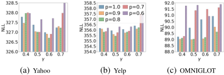
Parameter Analysis. Here, we train DU-VAE by varying γ from 0.4 to 0.7 and p from 1 to 0.6. As the Figure 2 shows, we find that, DU-VAE would achieve the best NLL with parameters (γ, p) as when (0.6, p = 0.8) for Yahoo, (0.5, p = 0.8) for Yelp, and (0.5, p = 0.9) for OMNIGLOT, respectively.
4.3 Case Study-Latent Space Visualization
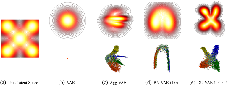
Here, we aim to provide one intuitive comparison of latent spaces learned by different models based on one simple synthetic dataset. Specifically, following [Kim et al., 2018], we first sample 2-dimensional latent variable z from one mixture of Gaussian distributions that have 5 mixture components. Then one text-like dataset can be generated from one LSTM layer conditioned on those latent variables. Based on this synthetic dataset, we trained different VAEs with 2dimensional standard Gaussian prior and diagonal Gaussian posterior. Then, we visualize the learned latent spaces by displaying the counter plot of the aggregated approximated posteriors q(z) = EpD(x)[qφ(z|x)] and the location of approximated posterior's mean parameters for different samples x.
According to the results in Figure 1, we have some interesting observations. First, due to the posterior collapse, VAE
learns an almost meaningless latent space where the posterior q(z|x) for all data are squeezed in the center. Actually, it is not surprising that the aggregated posterior matches the prior excessively in this case, because we almost have qφ(z|x) = p(z), ∀x. Second, Agg-VAE, BN-VAE, and DUVAE all tend to diverse samples in different categories, but in different manners and degrees. Intuitively, all three models force to embedding the blue category in the center around by the other four categories. However, only the average posterior learned by DU-VAE have five centers same as the true latent space. Meanwhile, DU-VAE with Dropout strategy encourages the aggregated posteriors to be more compact, while that of BN-VAE is more broad, compared with the prior. Those observations demonstrate that DU-VAE tends to guide the latent space to be more diverse and less uncertain.
5 Conclusion
In this paper, we developed a novel generative model, DUVAE, for learning a more diverse and less uncertain latent space. The goal of DU-VAE is to ensure that more meaningful and compact representations can be learned. Specifically, we first demonstrated theoretically that it led to better latent space with high diversity and low uncertainty awareness by controlling the distribution of posterior's parameters across the whole dataset respectively. Then, instead of introducing new loss terms or modifying training strategies, we proposed to apply Dropout on the variances and Batch-Normalization on the means simultaneously to regularize their distributions implicitly. Furthermore, we extended DU-VAE into VAEIAF empirically. The experimental results on three benchmark datasets clearly showed that DU-VAE outperformed state-of-the-art baselines on both likelihood estimation and underlying classification tasks.
Acknowledgements
This work was partially supported by grants from the National Natural Science Foundation of China (Grant No. 91746301, 61836013).
@inproceedings{ijcai2021p408,
  title     = {Regularizing Variational Autoencoder with Diversity and Uncertainty Awareness},
  author    = {Shen, Dazhong and Qin, Chuan and Wang, Chao and Zhu, Hengshu and Chen, Enhong and Xiong, Hui},
  booktitle = {Proceedings of the Thirtieth International Joint Conference on
               Artificial Intelligence, {IJCAI-21}},
  publisher = {International Joint Conferences on Artificial Intelligence Organization},
  editor    = {Zhi-Hua Zhou},
  pages     = {2964--2970},
  year      = {2021},
  month     = {8},
  note      = {Main Track},
  doi       = {10.24963/ijcai.2021/408},
  url       = {https://doi.org/10.24963/ijcai.2021/408},
}
TY - CPAPER TI - Regularizing Variational Autoencoder with Diversity and Uncertainty Awareness AU - Shen, Dazhong AU - Qin, Chuan AU - Wang, Chao AU - Zhu, Hengshu AU - Chen, Enhong AU - Xiong, Hui T2 - Proceedings of the Thirtieth International Joint Conference on Artificial Intelligence, IJCAI-21 PB - International Joint Conferences on Artificial Intelligence Organization PY - 2021 SP - 2964 EP - 2970 DO - 10.24963/ijcai.2021/408 UR - https://doi.org/10.24963/ijcai.2021/408 ER -Copied
Machine-readable versions of this paper, for tools and AI agents:





