
Explaining Deep Neural Network Models with Adversarial Gradient Integration
Proceedings of the Thirtieth International Joint Conference on Artificial Intelligence. Main Track. Pages 2876-2883.
https://doi.org/10.24963/ijcai.2021/396
Keywords
- AI Ethics, Trust, Fairness: Explainability
- Machine Learning: Explainable/Interpretable Machine Learning
- Machine Learning: Adversarial Machine Learning
Abstract
Deep neural networks (DNNs) have became one of the most high performing tools in a broad range
of machine learning areas. However, the multilayer non-linearity of the network architectures prevent
us from gaining a better understanding of the models’ predictions. Gradient based attribution
methods (e.g., Integrated Gradient (IG)) that decipher input features’ contribution to the prediction
task have been shown to be highly effective yet requiring a reference input as the anchor for explaining
model’s output. The performance of DNN model interpretation can be quite inconsistent with
regard to the choice of references. Here we propose an Adversarial Gradient Integration (AGI) method
that integrates the gradients from adversarial examples to the target example along the curve of steepest
ascent to calculate the resulting contributions from all input features. Our method doesn’t rely on
the choice of references, hence can avoid the ambiguity and inconsistency sourced from the reference
selection. We demonstrate the performance of our AGI method and compare with competing methods
in explaining image classification results. Code is available from https://github.com/pd90506/AGI.
- [Adadi and Berrada, 2018] Amina Adadi and Mohammed Berrada. Peeking inside the black-box: A survey on explainable artificial intelligence (xai). IEEE Access, 6:52138-52160, 2018.
- [Adebayo et al., 2018] Julius Adebayo, Justin Gilmer, Michael Muelly, Ian Goodfellow, Moritz Hardt, and Been Kim. Sanity checks for saliency maps. Advances in neural information processing systems, 31:9505-9515, 2018.
- [Chattopadhay et al., 2018] Aditya Chattopadhay, Anirban Sarkar, Prantik Howlader, and Vineeth N Balasubrama- nian. Grad-cam++: Generalized gradient-based visual ex- planations for deep convolutional networks. In 2018 IEEE Winter Conference on Applications of Computer Vision (WACV), pages 839-847. IEEE, 2018.
- [Datta et al., 2016] Anupam Datta, Shayak Sen, and Yair Zick. Algorithmic transparency via quantitative input in- fluence: Theory and experiments with learning systems. In 2016 IEEE symposium on security and privacy (SP), pages 598-617. IEEE, 2016.
- [Fong and Vedaldi, 2017] Ruth C Fong and Andrea Vedaldi. Interpretable explanations of black boxes by meaningful perturbation. In Proceedings of the IEEE International Conference on Computer Vision, pages 3429-3437, 2017.
- [Goodfellow et al., 2014] Ian J Goodfellow, Jonathon Shlens, and Christian Szegedy. Explaining and harnessing adversarial examples. arXiv preprint arXiv:1412.6572, 2014.
- [He et al., 2015] Kaiming He, Xiangyu Zhang, Shaoqing Ren, and Jian Sun. Deep residual learning for image recog- nition. corr abs/1512.03385 (2015), 2015.
- [Li et al., 2016] Jiwei Li, Will Monroe, and Dan Juraf- sky. Understanding neural networks through representa- tion erasure. arXiv preprint arXiv:1612.08220, 2016.
- [Li et al., 2020] Xiangrui Li, Xin Li, Deng Pan, and Dongx- iao Zhu. On the learning property of logistic and softmax losses for deep neural networks. In AAAI 2020, New York, NY, USA, February 7-12, 2020, pages 4739-4746. AAAI Press, 2020.
- [Lundberg and Lee, 2017] Scott M Lundberg and Su-In Lee. A unified approach to interpreting model predictions. In Advances in neural information processing systems, pages 4765-4774, 2017.
- [Madry et al., 2017] Aleksander Madry, Aleksandar Makelov, Ludwig Schmidt, Dimitris Tsipras, and Adrian Vladu. Towards deep learning models resistant to adversarial attacks. arXiv preprint arXiv:1706.06083, 2017.
- [Pan et al., 2020] Deng Pan, Xiangrui Li, Xin Li, and Dongxiao Zhu. Explainable recommendation via inter- pretable feature mapping and evaluation of explainability. In Christian Bessiere, editor, Proceedings of the Twenty- Ninth International Joint Conference on Artificial Intelli- gence, IJCAI 2020, pages 2690-2696. ijcai.org, 2020. IJCAI
- [Petsiuk et al., 2018] Vitali Petsiuk, Abir Das, and Kate Saenko. Rise: Randomized input sampling for explanation of black-box models. arXiv preprint arXiv:1806.07421, 2018.
- [Qiang et al., 2020] Yao Qiang, Xin Li, and Dongxiao Zhu. Toward tag-free aspect based sentiment analysis: A mul- tiple attention network approach. In 2020 International Joint Conference on Neural Networks, IJCNN 2020, Glas- gow, United Kingdom, July 19-24, 2020, pages 1-8. IEEE, 2020.
- [Ribeiro et al., 2016] Marco Tulio Ribeiro, Sameer Singh, and Carlos Guestrin. " why should i trust you?" explain- ing the predictions of any classifier. In Proceedings of the 22nd ACM SIGKDD international conference on knowl- edge discovery and data mining, pages 1135-1144, 2016.
- [Selvaraju et al., 2017] Ramprasaath R Selvaraju, Michael Cogswell, Abhishek Das, Ramakrishna Vedantam, Devi Parikh, and Dhruv Batra. Grad-cam: Visual explanations from deep networks via gradient-based localization. In Proceedings of the IEEE international conference on com- puter vision, pages 618-626, 2017.
- [Shrikumar et al., 2017] Avanti Shrikumar, Peyton Green- side, and Anshul Kundaje. Learning important features through propagating activation differences. In Proceed- ings of the 34th International Conference on Machine Learning-Volume 70, pages 3145-3153. JMLR. org, 2017.
- [Simonyan and Zisserman, 2014] Karen Simonyan and An- drew Zisserman. Very deep convolutional networks for large-scale image recognition. arXiv preprint arXiv:1409.1556, 2014.
- [Simonyan et al., 2013] Karen Simonyan, Andrea Vedaldi, and Andrew Zisserman. Deep inside convolutional networks: Visualising image classification models and saliency maps. arXiv preprint arXiv:1312.6034, 2013.
- [Springenberg et al., 2014] Jost Tobias Springenberg, Alexey Dosovitskiy, Thomas Brox, and Martin Ried- miller. Striving for simplicity: The all convolutional net. arXiv preprint arXiv:1412.6806, 2014.
- [Sundararajan et al., 2017] Mukund Sundararajan, Ankur Taly, and Qiqi Yan. Axiomatic attribution for deep net- works. arXiv preprint arXiv:1703.01365, 2017.
- [Szegedy et al., 2015] Christian Szegedy, Vincent Van- houcke, Sergey Ioffe, Jonathon Shlens, and Zbigniew Wojna. Rethinking the inception architecture for computer vision. corr abs/1512.00567 (2015), 2015.
- [Zhou et al., 2016] Bolei Zhou, Aditya Khosla, Agata Lapedriza, Aude Oliva, and Antonio Torralba. Learning deep features for discriminative localization. In Proceed- ings of the IEEE conference on computer vision and pat- tern recognition, pages 2921-2929, 2016.
References were extracted automatically from the PDF and may contain errors.
Full text extracted automatically from the PDF; figures, tables and equations may differ. The PDF is the version of record.
1 Introduction
Recently, deep neural networks (DNNs) has attracted much attention in machine learning community due to its state-ofthe-art performance on various tasks such as image classification [Li et al., 2020], sentiment analysis [Qiang et al., 2020] and item recommendation [Pan et al., 2020]. Despite the successes, interpreting a complex DNN still remains an open problem, hindering its wide deployment in safety and security-critical domains. A trustworthy DNN model should not only demonstrates a high performance in its detection and prediction, but also needs to explainable [Adadi and Berrada, 2018]. DNNs are complex nonlinear functions parameterized by model weights; understanding how the information flows from input to output remains a major challenge in Explainable Artificial Intelligence (XAI) research.
∗Corresponding author
In general there are two directions towards interpreting DNNs, i.e., gradient based methods, and local approximation methods. Some gradient based methods calculate input feature importance by exploiting its gradient with respect to the model inputs. For example, Saliency Map (SM) [Simonyan et al., 2013] uses gradient directly, Guided Backpropagation [Springenberg et al., 2014] only propagates non-negative gradients, and Integraded Gradients (IG) [Sundararajan et al., 2017] integrates gradients from a reference to input. Class Activation Mapping (CAM) based methods [Zhou et al., 2016; Selvaraju et al., 2017; Chattopadhay et al., 2018] capture the gradient with respect to intermediate layers of convolutional feature maps. As for the local approximation methods, extensive research have been done to explain the local neighborhood behaviors of a complex model by approximating it with a simple yet interpretable model [Ribeiro et al., 2016; Shrikumar et al., 2017; Lundberg and Lee, 2017], such as linear model and decision tree. Other methods such as [Fong and Vedaldi, 2017; Datta et al., 2016; Li et al., 2016] attempt to perturb the inputs to identify the part of inputs that are most responsible for a prediction in the neighborhood.
Within gradient models, although CAM based methods give promising results in various applications, a major limitation is that it applies only to Convolutional Neural Network (CNN) architectures. SM works on non-CNN models, however, it only captures the local gradient information at the inputs, which can be misleading due to the high non-linearity of DNNs. To overcome these limitations, methods such as IG [Sundararajan et al., 2017] are proposed to not only consider the gradients at the input, but also the cumulative gradients along the path from a reference to the input example.
One key issue of IG (as well as other methods such as DeepLIFT [Shrikumar et al., 2017]) is that it explicitly requires a reference (or baseline) to make interpretation. This could result in inconsistent interpretations with regard to different references. Although finding a reasonable reference is not infeasible for easier tasks (e.g. MNIST classification), it could become problematic when the underlying tasks are complicated. As described by the authors of IG paper : "a reference should convey a complete absence of signal". If both white noise image and black image convey no signal, why prefer the latter to the former in simpler tasks? Does it hold true for more complex tasks? In the DeepLIFT paper, a blurred version of the original input is used as the reference as opposed to a black image for CIFAR-10 data. As such, the choice of reference can be ad hoc and lack of rigorous justification.
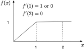
To tackle this major issue, we attempt to eliminate the requirement of reference by utilizing the false class gradients to find adversarial examples for the DNN classifier. A simple intuition is that adversarial examples are well-defined and easy to find given the input and the DNN model. In contrast, the choice of a reference can be more subjective and ad hoc. We derive our formulation based on the observation that sum of gradients from all classes equal to 0, as such, the false class gradients are equivalent to the gradient of the true class.
We summarize our main contributions as follows: 1) we propose a novel Adversarial Gradient Integration (AGI) method for a more consistent DNN model interpretation eliminating the need for a reference; 2) we establish the connection between the true class' and the false classes' gradients; and 3) we explain a DNN model's prediction via discriminating against the false classes, instead of focusing only on correct classification of the true class.
2 Preliminaries
To describe our approach, we first review gradient-based SM [Simonyan et al., 2013] and IG [Sundararajan et al., 2017] methods, and show their limitations such as gradient vanishing issue (Figure 1) and ad hoc choice of reference issue. In section 3 and 4, we derive our AGI method and show that it has various attractive properties that can overcome the limitation of the previous methods.
2.1 SaliencyMap
Saliency Map [Simonyan et al., 2013] is a pioneering visualization method for model interpretation, which simply calculates the gradient of classification output with respect to the input images. Formally, MSaliency = ∇xf t (x), where t represents the true label, and f t (x) represents the output value corresponding to the true class label. This method captures the local gradient information at the input, however, it can result in misleading interpretations since local gradient information may not faithfully represent the global attribution. For example, in Figure 1, the gradient at x = 2 is 0, however, we could not say that the contribution from x is none. Moreover, when x = 1, the gradient may be inconsistent, i.e., 1 or 0, depending on how we define the gradient. These critical issues need to be addressed.
2.2 Integrated Gradients
Different remedial methods have been developed to address the inconsistency among the local gradients shown in Figure 1. For example, DeepLIFT [Shrikumar et al., 2017] calculates the difference between x = 0 and x = 2 rather than using the gradient at one point. Another method to mitigate the drawbacks of SM is to integrate the gradient from x = 0 to x = 2 to average the effects. This strategy not only avoids the gradient vanishing issue, but also prevents the obstruction of some singular points (i.e., where gradient is not continuous), as long as the model is integrable within the range. In fact, this is similar to the idea of IG proposed by [Sundararajan et al., 2017]. The formulation of IG is
where j denotes the index of jth input feature, x′j represents a reference. Although IG successfully addresses the issues of SM method, we point out the following two limitations: 1) a predefined path is needed to integrate from a reference to the original input. IG takes a straight line specified by γ(α) = x′ + α × (x-x′ ) in the input space as the integrating path; and 2) a manually selected reference is required because integration must have a starting point.
3 ProblemFormulation
Looking into IG's first limitation: the predefined integrating path, one motivation of picking the straight line from a reference to the input is because it is the shortest path in the input space. Intuitively, to effectively discriminate the input from a reference point, an integration method should indeed pick the shortest path (if there are any detour, it may then contain information that discriminates from other examples). However, the problem is what we are interested is the learned feature space from the penultimate layer of DNNs, instead of the input space. Hence the shortest path needs to be the one in the learned feature space. As the mapping from input space to feature space is highly non-linear and complex, the corresponding curve, i.e., shortest curve, in the input space is most likely not a straight line.
The problem to solve becomes how can we find such a curve in the input space that may correspond to the shortest path in the feature space? Since operations from the penultimate layer to the output layer is usually linear, the shortest curve from the input point to a reference should correspond to a straight line in the feature space (Figure 2). Thanks to backpropagation method, as long as we find the gradient along the direction of the straight line in feature space, we are guaranteed to obtain the corresponding path in the input space. Assuming the last layer has parameter set W and the penultimate layer's output is φ(x), the output of the last layer is then y = Wφ(x). Taking the derivative with respect to φ(x), we have y′ = W, which corresponds to a constant gradient field. The steepest descent algorithm is guaranteed to find a straight line in a constant gradient field. Using chain rule in backpropagation, we obtain the gradient field in the input space, and hence the corresponding curve.
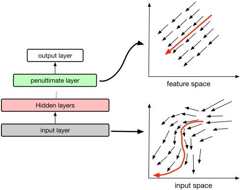
With respect to the second limitation: the choice of reference, from the above discussion, we actually have already observed the redundancy of the reference: although there should be a destination at the end of the straight line, we don't have to pre-define it. In such a case, the steepest descent algorithm can not only lead us to a candidate reference point, but also help us finding the shortest path. Hence both reference and integration path can be obtained with the model and inputs provided, and is input specific. Figure 2 illustrates the shortest paths in the feature space (right upper panel) and the input space (right lower panel). Note that the assumption of linearity from penultimate layer to output layer is not required since we can use steepest descent algorithm regardless.
The property of steepest descent appears to be flawless, however, the caveat arises from the inconsistency. i.e., ideally, just like the choice of the reference, the descent should lead us to a point where all class outputs being equal. Unfortunately, this usually isn't possible. The reason is that although we can control the descent of the true class, we have no control of which false class will ascend along the path. In fact, descending from the true class could very likely result in ascending to one of the false class instead of evenly distributed to all false class [Goodfellow et al., 2014].
4 Adversarial Gradient Integration
Here we formally describe the proposed AGI method to overcome the aforementioned limitations, i.e., the inconsistency in automatically finding the reference.
4.1 Perspective: Discrimination v.s. Classification
The discussion we have thus far motivates us to define a more consistent and systematic concept than the reference for IG based model explanation. Here we propose using adversarial example in lieu of reference. Unlike the latter whose definition can be vague thus ad hoc, a targeted adversarial example is clearly defined as the closest perturbed example to the original input such that it changes prediction of the true class to the targeted class(es).
To understand the rationale behind our choice, let's imagine in a classification task, instead of considering a prediction as classifying the input as the true class, why not view it as discriminating the input to all the false classes? Therefore, rather than interpreting what makes the model to classify the true class, we may equivalently interpret what makes the model to discriminate the true class from the false classes.
With the perspective of discrimination in mind, how could we leverage adversarial examples to reinforce the role that a reference plays? Recall in the discussion of gradient SM method, we have the property that all class probabilities are summed to 1, and we have the overall zero gradient, leading us to establish the connection between true class gradient and adversarial gradients as below:
It means that the gradient of the true class t w.r.t the input is equivalent to the summation of negative gradient of the false classes w.r.t the input. This inspires us that in the neighborhood of the input, the gradient contribution to the true class label and the adversarial class labels are equivalent.
Lets focus on one adversarial false class i, whose gradient we call as an adversarial gradient toward class i. If we follow the direction of the adversarial gradient, and perturb the input via ascending the gradient direction (i.e., x ← x+ϵ ·∇f i (x), the steepest ascent), over multiple steps, we may eventually approach a point where the perturbed input becomes an adversarial example x′(i) , which gives false prediction of class i instead of t.
In this case, lets assume that there is a path denoted by γ(α), what we are interested is how the true class prediction f t (x) changes along the path. And what is its role in making model interpretation? To understand these, let's first define the path gradient integration (PGI):
Definition 1. Assume f denotes the prediction model, f t is the true class output of the model. Let x be the original input, and x′ is another point in the input space. If there is a path γ(α) from x′ to x, with x′ = γ(0) and x = γ(1), the path gradient integration for the jth input feature is defined by
Definition 1 essentially defines a path integration from a starting point to the input point, following the path γ(α). If we define the starting point to be the choice of reference x′ , and take a straight line path from reference x′ to the input x, i.e. γ(α) = x′ + α × (x-x′ ), Definition 1 becomes an alternative formulation of IG [Sundararajan et al., 2017]:
But what if we use an adversarial example x′i as the starting point rather than a reference point? Following the interpretation of IG, which states that the result of IG represents the attribution of the input features to the prediction, similarly, we can interpret the integration from the adversarial example as the attribution of the input feature to discriminate the true class t from a false class i.
4.2 Adversarial Gradient Integration (AGI)
Integrating along a straight line from adversarial example x′i to x is not ideal. The shortest path in the input space doesn't account for the shortest path in learned feature space (as we discussed in Section 3). Hence here the steepest ascent path is chosen as the integration path.
Definition 2. Given all assumptions fromDefinition 1. Let f i be a false class output, γ(α) be the path obtained by steepest ascending f i , and x′i be the corresponding adversarial example at the end of the path, the adversarial gradient integration of the jth input feature is defined by
Recall that in [Sundararajan et al., 2017], the authors propose that an attribution method needs to satisfy three axioms, i.e., sensitivity, implementation invariance, and completeness. We argue AGI satisfies all of them due to the nature of path integration. From Definition 2, we can easily find that IG and AGI differ only in two aspects: 1) AGI integrates over the curve of steepest ascent whereas IG integrates over a straight line from the input space; and 2) AGI starts from an adversarial example, while IG starts from a manually selected reference point. The differences essentially are summarize to two benefits of AGI: 1) it gives more intuitive shortest path in the learned feature space, and 2) no need to manually select the reference point, preventing the derived inconsistency.
4.3 From IG to AGI
Follow the interpretation by IG: the IG result shows the contribution of individual input features to the true class t. We interpret AGI similarly as: the AGI result shows the attribution of individual input feature to discriminate t from a false class i. Now, what if we sum AGIs from all false classes? Inspired by Eq. 2, we assume
which essentially says that the attribution to all discriminations should be equivalent to attribution to classification. The rationale is that although we usually say that a model classifies the input as something, another perspective can be, in contrast, that a model discriminates something from other things. For example, LeNet discriminates one digit class from other digit classes in MNIST dataset. Hence we can interpret a classification by summing over all interpretations of AGIs, which essentially interprets the discrimination between all adversarial classes and the true class.
Algorithm 1: IndividualAGI(f, x, i, ϵ, m)
Input : Classifier f, input x, adversarial class i step size ϵ, max number of steps m;
Output: Individual AGI for class i: AGIi; AGIi ← 0; j ← 0 ; while argmaxℓ f ℓ (x) ̸= i and j < m do end4.4 Finding the Steepest Ascending Path
In order to obtain AGI for one false class i, two gradients need to be calculated: ∇xf i (x) and ∇xf t (x). Note that because the path is defined by steepest ascent, then in Eq. 5, we have
the minus sign here is because the direction is opposite (we ascend from x to x′i , while integration is done from x′i to x). The formulation then becomes
which integrates along the path until argmaxℓ f ℓ (x) = i Here we may face the issue that gradient ascending may encounter local maxima that prevents it from ascending further. We adopt the approach proposed by [Madry et al., 2017] that uses the signed gradient instead of the original gradient to make sure it is easier to surpass the decision boundary. In addition, we set a maximum step size m to prevent the path from infinite looping when trapped in local maxima. The algorithm for computing individual AGI is given by Algorithm 1 (the subscript j is omitted for conciseness).
4.5 Individual AGI Aggregation
As for aggregating all individual AGIs, when the number of classes are small, we can simply sum up all AGIs. However, when there are a large amount of classes, such as 1000 classes in ImageNet dataset, calculating all AGIs for 999 false classes become computational prohibitive. In order to alleviate the excessive computational burden, we randomly select a reasonable amount of false classes by sampling from all candidate classes. Although this sampling procedure may lose information from the unselected classes, the resulting AGI can still capture the essential information because the discriminating tasks actually share a fair amount of semantic information. For example, the information for discriminating Labrador from Cat may be similar to discriminating Shepherd from Cat. Hence we argue that sampling a subset of classes is adequate to obtain a satisfying model interpretation and we also provide experimental justifications in Section 5.3 and Section 5.4. The algorithm for calculating AGI is given by Algorithm 2.
Algorithm 2: AGI(f, x, ϵ, k, m) Input : Classifier f, input x, step size ϵ, subsampling size k, max number of steps m; Output: AGI; AGI ← 0; S ← Sampling k false classes ; for i in S do AGI ← AGI + IndividualAGI(f, x, i, ϵ, m) end5 Experiments
In this section, we perform experiments attempting to answer the following questions: 1) does AGI output meaningful interpretations for classifying the true class? 2) does class subsampling compromise the performance? 3) does individual AGI give reasonable interpretation for discriminating the true class against a false class? and 4) does AGI pass sanity checks?
5.1 Experimental Setup
The model to be interpreted includes InceptionV3 [Szegedy et al., 2015], ResNet152 [He et al., 2015] and VGG19 [Simonyan and Zisserman, 2014]. All experiments are conducted using ImageNet dataset.
In terms of baseline DNN interpretation methods, we use SM [Simonyan et al., 2013] and IG[Sundararajan et al., 2017] as baselines for qualitative and quantitative comparisons of interpretation quality. Additionally, Guided-Backpropagation [Springenberg et al., 2014] is selected for comparison with AGI in the sanity check experiments. Regarding parameter settings, we set the step size ϵ = 0.05, and the class subsampling size for ImageNet to 20. As for the reference for IG method, we use the default choice in the original paper (i.e., black image).
Additional data processing to optimize the heatmap visualization have also been used. We reassign all heatmap attributions less than q = Percentile(80%) to be q (lower bound), and all values larger than u = Percentile(99%) to be u (upper bound), then normalize them within [0, 1]. The lower bound is set because that we only want to focus on the area with relatively high attributions, a low attribution is likely caused by background. The upper bound is set to avoid extremely high values that can potentially undermine the visualization (This procedure is applied to all methods).
Our implementation for generating the steepest ascent curve is inspired from the PGD attack algorithm [Madry et al., 2017]. For InceptionV3, setting the max ascending step = 20, and sample size = 20, it will cost ≈ 15 seconds to interpret a single 224 × 224 color image on a computer with Nvidia GTX 1080 GPU. However, the path-finding procedure for sampled negative classes can be paralleled to speed up the running time, making the overall process less than 1 second.
5.2 Qualitative Evaluation
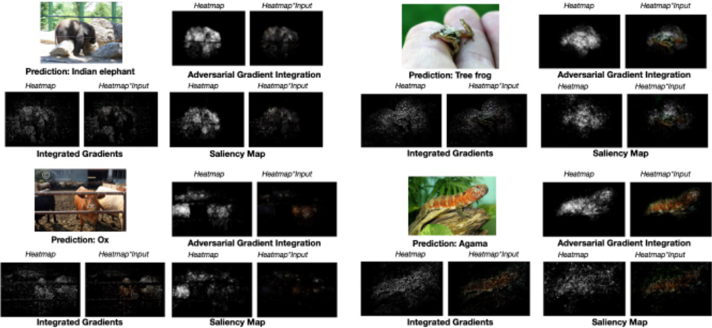
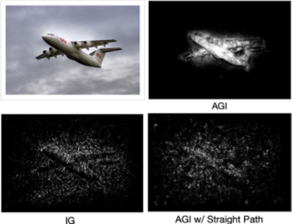
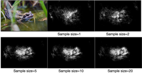
Figure 3 shows examples of different interpretation methods explaining predictions made by InceptionV3 (Additional examples and experiments on Resnet152 and VGG19 can be found in the supplementary materials). A key observation from the experiments is that IG's output heatmap is far more sparse than AGI's (by sparse, we mean high attribution values are sparsely distributed in the map instead of concentrating on the target objects). We argue that this phenomenon is sourced from two aspects: First, IG uses a black image as the default reference whereas AGI doesn't. Black reference image may be good for those cases where objects are light colored, but can fail when the target object is dark. For example, the heatmap of Indian Elephant generated by IG (Figure 3) doesn't highlight the body of the elephant which is in fact under the shadow whereas that generated by our AGI has no such issue. Second, IG uses shortest integration path (straight line) in input space whereas AGI uses shortest path in the learned feature space. To demonstrate the relationship between the straightline integration and sparsity, we replace our AGI's integration path with the straight line, i.e., instead of integrating over the curve of steepest ascent, we integrate from adversarial examples to the input example over a straight line like IG. The results in Figure 4 show that an inappropriate integration path may cause heatmap sparsity.
5.3 Quantitative Evaluation
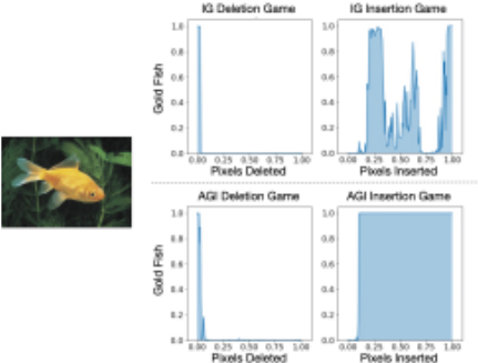
In addition to the qualitative examples presented above, we also conduct quantitative experiments to validate our method using insertion scores and deletion scores [Petsiuk et al., 2018]. Starting from a blank image, the insertion game successively inserts pixels from highest to lowest attribution scores and makes predictions. We draw a curve that represents the prediction values, the area under the curve (AUC) is then defined as the insertion score. The higher the insertion score, the better the quality of interpretation. Similarly, starting from the original image, the deletion score is obtained by successively deleting the pixels from the highest to lowest attribution scores. The lower the deletion score, the better the quality of interpretation. An example of such process is shown in Figure 5. Table 1 shows the average scores over 1000 test examples in ImageNet by InceptionV3 and ResNet152.
| Metrics | Deletion Score | Insertion Score | ||||||||||
|---|---|---|---|---|---|---|---|---|---|---|---|---|
| Methods | IG | SM | AGI-1 | AGI-5 | AGI-10 | AGI-20 | IG | SM | AGI-1 | AGI-5 | AGI-10 | AGI-20 |
| InceptionV3 | 0.032 | 0.036 | 0.043 | 0.043 | 0.046 | 0.048 | 0.294 | 0.537 | 0.408 | 0.503 | 0.532 | 0.561 |
| ResNet152 | 0.030 | 0.056 | 0.044 | 0.052 | 0.056 | 0.060 | 0.262 | 0.407 | 0.405 | 0.475 | 0.489 | 0.503 |
While IG, SM and AGI all have sufficiently small deletion scores (Note that deletion score become less indicative when getting extremely small due to the existence of adversarial effects in DNNs [Petsiuk et al., 2018]). AGI has much larger insertion scores than the competitors (Table 1). Since the latter is an indicator of the ability to detect the target object, we conclude that AGI outperforms IG and SM in terms of detecting the meaningful objects. Observing the trend from AGI-1 to AGI-20, the insertion score converges when the subset of selected false classes become sufficiently large. In the case of InceptionV3, fromAGI-1 to AGI-10, the insertion score gain per additional class is ∼ 0.014 whereas the score gain per additional class become ∼ 0.003 from AGI-10 to AGI-20. This demonstrates that a relatively small subset of false classes is sufficient to obtain a good interpretation.
5.4 Class Subsampling
A major computational burden of our AGI method is to calculate individual AGI for all false classes. As we argued before, random subsampling doesn't affect the results as long as the sample size is sufficiently large. Although individual AGIs may be different for different false classes, the aggregated AGI converges when sample size increases. As such, the information from the sampled AGIs is sufficient to generalize to all other classes. Figure 6 substantiates our claim: the results indeed become more clear when sample size increases from 1 to 10 but doesn't change too much afterwards. This observation indicates that different discriminating tasks may share a fair amount of input attributions, hence a small subset can be sufficiently representative for the overall interpretation. Note that it is possible to utilize the semantic information to help selecting the subset of classes, which could render better results. We didn't utilize it for subsampling in this paper mainly because that the random selection method can already output promising results. However, we do point out that utilizing semantic information for subsampling process may potentially reduce the sampling size.
5.5 Discrimination fromOther Classes
One of our main contributions is that we decompose the interpretation of classifying the true label into the sum of interpretation of discriminating against false labels. To demonstrate our claim, we conduct experiments to interpret model discrimination using individual AGIs (Algorithm 1). The individual AGI should represent the attributions that discriminate true class from the specific false class.
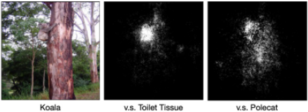
Figure 7 shows an example from ImageNet dataset. To discriminate Koala from Toilet Tissue, we can observe that only the body of Koala from the image is highlighted in the heatmap. However, when attempting to discriminate it from a Polecat, the attribution from the trunk become more prominent, which means the latter is used to reinforce explanation. The underlying reason behind it could be that Polecats don't live on trees, while Koala do.
5.6 Sanity Checks for Image Interpretation
As pointed out by [Adebayo et al., 2018], visual interpretation could be misleading, as some previous interpretation methods are just edge detection instead of genuine interpretation. In case when an interpretation method is independent of either the prediction model or of the data generating process, a sanity check is required for validating its correctness.
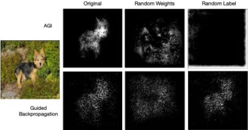
Here we perform two tests for the sanity check, 1) a model parameter randomization test: the interpretation of model with learned parameters should be substantially different from the model with random parameters; and 2) a data randomization test: the same input with different labeling should result in different interpretations. Figure 8 shows that our AGI method passes both tests (first row) since after both model randomization and data randomization, the outputs are significantly different from the original ones. While GuidedBackpropagate [Springenberg et al., 2014] (second row), on the other hand, doesn't pass the data randomization test, as randomizing data label should has significant heatmap differences from the correct label (the heatmap corresponding to 'original' and 'random' labels).
6 Conclusion
In this paper, motivated by the limitations of two wellestablished DNN interpretation methods, SM and IG, we propose a novel attribution method, i.e., AGI, which doesn't require a manually selected reference, nor a predefined integration path. As such it can be applied to automatically and consistently explain DNNs' predictions. Through extensive experiments, our AGI method significantly outperforms the competing methods in both qualitative and quantitative experiments. Our AGI method can be broadly applied to explain a wide range of DNN models' predictions.
Acknowledgements
This work is supported by the National Science Foundation under grants CNS-2043611 and IIS-1724227.
Ethical Impact
DNN models have been increasingly deployed in many security and safety-critic real world settings. Despite the impressive performance, they are mostly black-box models that usually fail to give insight on why and how they make predictions. As trustworthiness and transparency become more salient issues, interpretable DNN methods are highly desirable and their wide adoption is expected to accelerate our current pace of leveraging AI for social good.
@inproceedings{ijcai2021p396,
  title     = {Explaining Deep Neural Network Models with Adversarial Gradient Integration},
  author    = {Pan, Deng and Li, Xin and Zhu, Dongxiao},
  booktitle = {Proceedings of the Thirtieth International Joint Conference on
               Artificial Intelligence, {IJCAI-21}},
  publisher = {International Joint Conferences on Artificial Intelligence Organization},
  editor    = {Zhi-Hua Zhou},
  pages     = {2876--2883},
  year      = {2021},
  month     = {8},
  note      = {Main Track},
  doi       = {10.24963/ijcai.2021/396},
  url       = {https://doi.org/10.24963/ijcai.2021/396},
}
TY - CPAPER TI - Explaining Deep Neural Network Models with Adversarial Gradient Integration AU - Pan, Deng AU - Li, Xin AU - Zhu, Dongxiao T2 - Proceedings of the Thirtieth International Joint Conference on Artificial Intelligence, IJCAI-21 PB - International Joint Conferences on Artificial Intelligence Organization PY - 2021 SP - 2876 EP - 2883 DO - 10.24963/ijcai.2021/396 UR - https://doi.org/10.24963/ijcai.2021/396 ER -Copied
Machine-readable versions of this paper, for tools and AI agents:





