
Multi-Cause Effect Estimation with Disentangled Confounder Representation
Proceedings of the Thirtieth International Joint Conference on Artificial Intelligence. Main Track. Pages 2790-2796.
https://doi.org/10.24963/ijcai.2021/384
Keywords
- Machine Learning: Explainable/Interpretable Machine Learning
- AI Ethics, Trust, Fairness: Trustable Learning
Abstract
One fundamental problem in causality learning is to estimate the causal effects of one or multiple treatments (e.g., medicines in the prescription) on an important outcome (e.g., cure of a disease). One major challenge of causal effect estimation is the existence of unobserved confounders -- the unobserved variables that affect both the treatments and the outcome. Recent studies have shown that by modeling how instances are assigned with different treatments together, the patterns of unobserved confounders can be captured through their learned latent representations. However, the interpretability of the representations in these works is limited. In this paper, we focus on the multi-cause effect estimation problem from a new perspective by learning disentangled representations of confounders. The disentangled representations not only facilitate the treatment effect estimation but also strengthen the understanding of causality learning process. Experimental results on both synthetic and real-world datasets show the superiority of our proposed framework from different aspects.
- [Hassanpour and Greiner, 2019] Negar Hassanpour and Russell Greiner. Learning disentangled representations for counterfactual regression. In International Conference on Learning Representations, 2019.
- [Higgins et al., 2016] Irina Higgins, Loic Matthey, Arka Pal, Christopher Burgess, Xavier Glorot, Matthew Botvinick, Shakir Mohamed, and Alexander Lerchner. Beta-vae: Learning basic visual concepts with a constrained varia- tional framework. 2016.
- [Hill, 2011] Jennifer L Hill. Bayesian nonparametric mod- eling for causal inference. Journal of Computational and Graphical Statistics, 20(1), 2011.
- [Jang et al., 2016] Eric Jang, Shixiang Gu, and Ben Poole. Categorical reparameterization with gumbel-softmax. arXiv preprint arXiv:1611.01144, 2016.
- [Lechner, 2001] Michael Lechner. Identification and estima- tion of causal effects of multiple treatments under the con- ditional independence assumption. In Econometric evalu- ation of labour market policies. 2001.
- [Li et al., 2017] Jundong Li, Kewei Cheng, Suhang Wang, Fred Morstatter, Robert P Trevino, Jiliang Tang, and Huan Liu. Feature selection: A data perspective. ACM Comput- ing Surveys (CSUR), 50(6), 2017.
- [Locatello et al., 2019] Francesco Locatello, Stefan Bauer, Mario Lucic, Gunnar Raetsch, Sylvain Gelly, Bernhard Schölkopf, and Olivier Bachem. Challenging common assumptions in the unsupervised learning of disentangled representations. In International Conference on Machine Learning, 2019.
- [Lopez et al., 2017] Michael J Lopez, Roee Gutman, et al. Estimation of causal effects with multiple treatments: a review and new ideas. Statistical Science, 32(3), 2017.
- [Louizos et al., 2017] Christos Louizos, Uri Shalit, Joris M Mooij, David Sontag, Richard Zemel, and Max Welling. Causal effect inference with deep latent-variable models. In Advances in Neural Information Processing Systems, 2017.
- [Ma et al., 2019] Jianxin Ma, Chang Zhou, Peng Cui, Hongxia Yang, and Wenwu Zhu. Learning disentangled representations for recommendation. In Advances in Neu- ral Information Processing Systems, 2019.
- [Rosenbaum and Rubin, 1983] Paul R Rosenbaum and Don- ald B Rubin. The central role of the propensity score in observational studies for causal effects. Biometrika, 70(1), 1983.
- [Rubin, 2005] Donald B Rubin. Bayesian inference for causal effects. Handbook of Statistics, 25, 2005.
- [Saini et al., 2019] Shiv Kumar Saini, Sunny Dhamnani, Akil Arif Ibrahim, and Prithviraj Chavan. Multiple treat- ment effect estimation using deep generative model with task embedding. In The World Wide Web Conference, 2019. [Schnabel, 2016] Schnabel. Recommendations as treat- ments: Debiasing learning and evaluation. In International Conference on Machine Learning, 2016.
- [Shalit et al., 2017] Uri Shalit, Fredrik D Johansson, and David Sontag. Estimating individual treatment effect: gen- eralization bounds and algorithms. In International Con- ference on Machine Learning, 2017.
- [Sharma et al., 2020] Ankit Sharma, Garima Gupta, Ran- jitha Prasad, Arnab Chatterjee, Lovekesh Vig, and Gautam Shroff. Multimbnn: Matched and balanced causal inference with neural networks. arXiv preprint arXiv:2004.13446, 2020.
- [Tran et al., 2017] Luan Tran, Xi Yin, and Xiaoming Liu. Disentangled representation learning gan for pose- invariant face recognition. In IEEE Conference on Com- puter Vision and Pattern Recognition, 2017.
- [Vemuri, 2015] Vijay K. Vemuri. Causal inference for statis- tics, social, and biomedical sciences: An introduction by guido w. imbens and donald b. rubin. Journal of Infor- mation Technology Case & Application Research, 17(3-4), 2015.
- [Wang and Blei, 2019] Yixin Wang and David M Blei. The blessings of multiple causes. Journal of the American Sta- tistical Association, 114(528), 2019.
- [Wang et al., 2018] Yixin Wang, Dawen Liang, Laurent Charlin, and David M Blei. The deconfounded recom- mender: A causal inference approach to recommendation. arXiv preprint arXiv:1808.06581, 2018.
- [Wang et al., 2020] Xiang Wang, Hongye Jin, An Zhang, Xi- angnan He, Tong Xu, and Tat-Seng Chua. Disentangled graph collaborative filtering. In International ACM SIGIR Conference on Research and Development in Information Retrieval, 2020.
- [Willmott and Matsuura, 2005] Cort J Willmott and Kenji Matsuura. Advantages of the mean absolute error (mae) over the root mean square error (rmse) in assessing aver- age model performance. Climate Research, 30(1), 2005.
- [Yoon et al., 2018] Jinsung Yoon, James Jordon, and Mi- haela van der Schaar. Ganite: Estimation of individu- alized treatment effects using generative adversarial nets. In International Conference on Learning Representations, 2018.
- [Zanutto et al., 2005] Elaine Zanutto, Bo Lu, and Robert Hornik. Using propensity score subclassification for mul- tiple treatment doses to evaluate a national antidrug media campaign. Journal of Educational and Behavioral Statis- tics, 30(1), 2005.
- [Zhang et al., 2019] Linying Zhang, Yixin Wang, Anna Os- tropolets, Jami J Mulgrave, David M Blei, and George Hripcsak. The medical deconfounder: Assessing treat- ment effects with electronic health records. In Machine Learning for Healthcare Conference, 2019.
- [Zhang et al., 2020] Weijia Zhang, Lin Liu, and Jiuyong Li. Treatment effect estimation with disentangled latent fac- tors. arXiv preprint arXiv:2001.10652, 2020.
References were extracted automatically from the PDF and may contain errors.
Full text extracted automatically from the PDF; figures, tables and equations may differ. The PDF is the version of record.
1 Introduction
One major challenge of causal effect estimation is the existence of unobserved confounders [Rosenbaum and Rubin, 1983], i.e., the unobserved variables which influence both treatment assignment and outcomes [Shalit et al., 2017]. Unobserved confounders can cause confounding bias to the estimated treatment effect. A line of recent studies infers unobserved confounders by modeling how instances are assigned with different treatments together. The problem is known as the multiple treatment effect (MTE) estimation [Wang and Blei, 2019]. A typical example is to estimate how intervening the cast of movies would change their potential revenues, e.g., "how much does the revenue (outcome) increase or decrease if Oprah Winfrey is in the movie?". Here, the genre of the movie is an unobserved confounder that affects which actors would star the movie as well as the revenue; and different actors in the cast (multiple treatment assignment) can provide complementary insights in revealing the movie genre.
∗Corresponding Author.
unobserved confounders by learning their latent representations [Wang and Blei, 2019; Saini et al., 2019] through the interactions between instances and treatments. However, the interpretability of the learned representations is limited, which could be an unknown mixture of several latent confounders' representations. In the movie cast example, the movie genre can be an unobserved confounder, but establishing the connection between this unobserved confounder and a particular part of the learned representations is difficult. In fact, it can greatly facilitate the human understanding of the confounding bias by separating the distinct, informative factors of variations in the confounders' representations [Locatello et al., 2019]. Motivated by the recent progress of disentangled representation learning [Higgins et al., 2016; Tran et al., 2017] which learns factorized representations of the independent data generative factors, we investigate the MTE estimation problem from a new perspective by learning disentangled representations for confounders to improve the interpretability of causality learning.
However, learning disentangled representations of confounders for MTE estimation remains nascent due to the following challenges: (1) Different latent confounders are not only mixed together but also can exhibit hierarchical patterns (e.g., high-level latent confounders such as "the movie is an animation movie" and low-level latent confounders like "the animation movie is from Disney"), which further increases the complexity of disentangled representation learning. (2) When estimating the treatment effects, most existing works take different treatments separately [Lopez et al., 2017] (i.e., constructing a prediction model for each treatment), which cannot capture the inherent dependencies between different treatments (e.g., two treatments could be similar if many instances are assigned with them simultaneously).
To address these challenges, we propose DIRECT - a novel framework of Disentangled multIple tReatment EffeCT estimation with the following desiderata: (1) To capture the hierarchical patterns of mixed confounders, we propose to disentangle the representations of latent confounders at two different levels. We first assume that treatments can be grouped into different clusters, as observed in many real-world scenarios [Schnabel, 2016]. Then by separately inferring confounders from the interactions between instances and each cluster of treatments (e.g., comedy actors or action actors), the learned confounder representations will become disentangled at the macro-level. Meanwhile, at the micro-level, we force different dimensions of the learned confounder representations to capture isolated factors with a carefully designed variational autoencoder (VAE) framework. (2) To tackle the issue that different treatments are often processed separately, we jointly consider multiple treatments simultaneously by leveraging their inherent dependencies. Specifically, we learn a trainable function to obtain the representation for each treatment based on treatment assignments. One appealing byproduct is that the framework can be generalized to new treatments that are not in the training data. Our main contributions include: 1) Problem: We formulate a new problem of disentangled multiple treatment effect estimation; 2) Framework: We propose a novel framework DIRECT to address this problem by learning disentangled confounder representations at two granularity levels; 3) Experiments: We conduct extensive experiments to show the superiority of DIRECT w.r.t. MTE estimation and interpretability.
2 ProblemDefinition
We use {A, Y } to denote the observational data, where A = {ai}ni=1 denotes the treatment assignment, and ai = {ai,j}mj=1 refers to the assignment of m different treatments on the i-th instance. Without loss of generality, we focus on treatments with binary values, i.e., ai,j ∈ {0, 1}. The observed outcome is denoted by Y = {yi}ni=1 , and yi ∈ R. We build our framework upon the potential outcome framework [Vemuri, 2015]. We represent the potential outcome in the multiple treatment setting by Ya = {yi(a)}ni=1 , where yi(a) is the value of the outcome that would be observed if the i-th instance receives the treatment assignment a ∈ {0, 1}m. Then the ITE for the i-th instance over a is defined as τi,a = yi(a) - yi(0), where yi(0) refers to the potential outcome when no treatment is assigned to the i-th instance.
Definition 1. (Disentangled multiple treatment effect estimation) Given observational data {A, Y }, our goal is to: (1) learn disentangled representations for the latent confounders. (2) estimate the ITE τi,a for each instance i under any treatment assignment a.
In our work, we relax the strong ignorability assumption [Rosenbaum and Rubin, 1983] (i.e., no unobserved confounders) by assuming that there may exist confounders Z = {z1, ..., zn} which (might be unobserved) can causally influence A and Y . Conditioning on the confounders, the treatment assignment is randomized, i.e., Yi(a) ⊥⊥ Ai|Zi 1 for any treatment assignment a ∈ {0, 1}m. Following [Wang and Blei, 2019], we also assume that for each instance i, the assignment of different treatments is independent with each other conditioned on the confounders, i.e., Ai,1 ⊥⊥ ... ⊥⊥ Ai,m|Zi. Other assumptions in this work include the Positivity, Consistency, and SUTVA assumptions [Rubin, 2005], which are widely-adopted in causal inference.
1 We use non-italicized capital letters to denote random variables, and italicized letters to denote specific realization. Among the italicized letters, non-bold letters denote scalars, bold lowercase letters denote vectors, and bold uppercase letters denote matrices or sets. For example, Zi is a randomly chosen vector of confounders, Z is the set which contains confounders of all instances, and zi denotes the values of confounders for instance i.
3 The Proposed Framework
The causal graph of the studied problem is shown in Fig. 1, where Zi denotes the confounders which influence the outcome and the assignment of at least one treatment for each instance i. Our framework DIRECT learns disentangled representations of confounders Z with a carefully designed variational autoencoder (VAE) architecture. At the macro-level, we learn the embedded cluster structure of different treatments to better learn and interpret the confounder representations. At the micro-level, we force each dimension of the learned representation to capture an isolated factor. Furthermore, by leveraging the dependencies among treatments, we learn a parameterized function to obtain the representation of each treatment. In this way, the model can be generalized to estimate the effects of treatment assignment including new treatments without retraining from scratch.
3.1 Model Description
Our framework includes three sets of latent variables: Z, T , and C, where T = {tj}mj=1 is the representation of treatments, C = {cj}mj=1 is the cluster assignment of the treatments, each cj is an one-hot vector and cj,k = 1 denotes that treatment j belongs to cluster k. As shown in Fig. 1, the distribution p(A, C, T, Z) can be factorized as:
where Θ = {A,C,T, Z}. Assume that the treatments can be divided into K clusters, we then divide the treatment assignments into K groups corresponding to the treatment clusters. The confounders are learned separately for the treatment assignments in each group for a macro-level disentanglement. The confounder representation learned from the assignment of treatments in cluster k is denoted by Z(k) = {z(k) 1 , z(k) 2 , ..., z(k) n }. Each Z(k) i is assumed to follow an isotropic unit Gaussian prior: Z(k) i ∼ N(0, I). Thus the distribution in Eq. (1) can be further factorized as:
An illustration of the proposed framework DIRECT is shown in Fig. 2, which follows a classical VAE architecture with the inference network and the generation network. The inference network infers the variational distributions of treatments and confounders based on the treatment assignment. The generation network reconstructs the input (i.e., treatment assignment), and predicts the potential outcome of each instance.
3.2 Inference Network
Since the true posterior distribution of the latent variables q(Z,T,C|A) is intractable, we use an inference network to Z"
A",%
A",&
……
Y"
),*-1
A
A",(
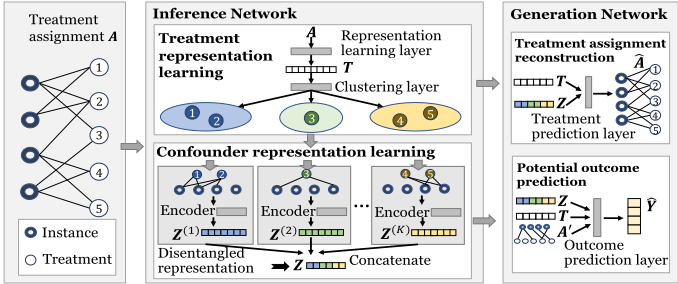
Figure 2: An illustration of the proposed framework DIRECT. It consists of two essential components: inference network and generation network.
approximate it based on the mean-field approximation. The approximate posterior q(Z, T, C|A) can be factorized as:
We learn the representations of treatments and confounders through the variational inference mentioned above, where ∗ represents all the indices, e.g., ai,∗ refers to ai,1, ..., ai,m.
Treatment Representation Learning
The proposed framework explicitly learns the treatments' representations from the observed treatment assignments. Specifically, the inference network specifies the form of the variational distributions of Tj to be Gaussian posteriors: q(Tj|a∗,j) = N(µT (a∗,j), diag(σ2T (a∗,j))). In the inference network, the mean and variance of the posterior are inferred by two separate neural network modules µT (·) and σT (·). We assume that the representations of treatments in the observational data have an inherent cluster structure composed with K components, where K is a hyperparameter. A clustering module is introduced in the inference network to approximate the cluster distribution q(Cj|tj) = Mult(fc(tj)), where fc(·) is a function of the clustering module. The output of fc(·) is a K-dimensional vector, where each element inside corresponds to the probability that the treatment belongs to each cluster. And the multinoulli distribution is implemented by a softmax layer. To enable clustering, the inference network specifies the prior of Tj to be N (µcj , diag(σ2 cj )), where µcj and σcj are parameters to be learned, referring to the mean and variance of the distribution of treatments in the cluster containing the j-th treatment. As the latent variable Cj is discrete, the reparameterization trick based sampling is not differentiable for backpropagation, thus we apply Gumbel-Softmax sampling [Jang et al., 2016] to approximate samples from the categorical distribution.
The treatment representation learning module enables the model to handle unseen treatments. For a new treatment m + 1, we can obtain its representation tm+1 and predict its cluster based on its treatment assignments and the trained model. Then, the potential outcome of those treatment assignments which involve the new treatment can be predicted with tm+1 and the learned confounder representations.
Disentangled Confounder Representation Learning
Inspired by [Ma et al., 2019], we learn disentangled representations of the confounders at two different levels. At the macro-level, the treatment assignment is divided into K groups according to the sampled C. We learn the representation Z(k) of confounders from each group k separately, and the final representation Z is the concatenation of Z(1) , ...,Z(K) . Specifically, the learned Zk is expected to correspond to the treatments in cluster k. For each Zk , we infer the posteriors distributions as: q(Z(k) i |ai,∗) = q(Z(k) i |a(k) i,∗ ) = N (µI (a(k) i,∗ ), diag(σ2 I (a(k) i,∗ ))), where a(k) i,∗ is the i-th instance's treatment assignment which only contains the treatments in cluster k. µI(·) and σI(·) are two neural network modules to infer the mean and variance of the distribution of q(Z(k) i |a(k) i,∗ ), respectively. At the micro-level, to achieve disentanglement among dimensions of learned representations, we specify a weight β ≫ 1 for the Kullback-Leibler (KL) divergence between the isotropic unit Gaussian prior and the learned distribution of each Z(k) to encourage the dimensions to reflect isolated latent factors.
3.3 Generation Network
In the generation model, we reconstruct the treatment assignment with a neural network module fa: p(Ai,j|zi, tj, cj) = Ber(sigmoid(fa(cj , zi, tj ))). We use a sigmoid layer to map the output of network fa(·) into (0, 1) as the probability of taking the treatment ai,j. In order to better capture the latent confounders, we also use the observed outcomes as a supervision signal. Specifically, we use a neural network module fy(Zi,Ai,T) to predict the potential outcome yi(a) for any treatment assignment a. We assume the prediction ˆYi(a) follows the Gaussian distribution N(yi(a), σ2 e ), where σ2 e is the variance of the prediction error. We use the observed outcome yi as target and minimize the outcome prediction loss: Ly = - ∑ni=1 log p( ˆYi = yi|zi, ai, T ).
3.4 Optimization
Following the classical VAE schema, the evidence lower bound (ELBO) LELBO can be derived as (the subscript q denotes q(Z,T,C|A) by default, and we drop the instance index i and treatment index j for notation simplicity):
| Dataset | Synthetic | Amazon-3C | Amazon-6C |
|---|---|---|---|
| # of instances | 2, 500 | 3, 000 | 6, 000 |
| # of treatments | 500 | 104 | 325 |
| # of clusters | 4 | 3 | 6 |
| Avg ratio of treated | 42.3% | 21.4% | 18.6% |
The ELBO consists of the reconstruction term and the KL term, which contains three terms: 1) the clustering prior term, where we use the uniform prior; 2) the treatment prior term, which drives the treatment clustering as described in the section of treatment representation learning; 3) the confounder prior term, which leads to disentanglement among dimensions by utilizing the isotropic nature of the prior. It is impractical to calculate the expectations over the variational distribution analytically, thus these terms are instead estimated by Monte Carlo samples from q(Z,T,C|A). By putting all the aforementioned components together, we obtain the loss function of the proposed framework:
Hyperparameters β and λ are used to control the effect of different parts of the objective function.
4 Experiments
4.1 Datasets
We evaluate the proposed method on one synthetic dataset and two semi-sythetic datasets from real-world scenarios. The detailed statistics of these datasets are shown in Table 1, including the number of instances, treatments, treatment clusters, and the average ratio of treatments assigned to instances.
Synthetic Dataset. We first conduct experiments on a synthetic dataset. This dataset is generated as follows:
i tj)), (6)
where i = 1, ..., n and j = 1, ...,m, π is a K-dimensional vector, corresponding to the probability that the treatment belongs to each cluster. We set dI (the dimension of each z(k) i )
and dT (the dimension of Tj) both as 20. The potential outcome of instance i under a treatment assignment a is simulated as yi(a) = aT TW1zi, where zi is the concatenation of z(k) i (k = 1, ...,K), and T = [t1, ..., tm]T . W1 is a matrix of parameters with dimensions dT × KdI .
Real-world Datasets. It is notoriously hard to obtain the ground truth treatment effect as we only observe one of the potential outcomes for each instance. Thus, we create two semi-synthetic datasets (Amazon-3C and Amazon-6C) based on the real-world Amazon review data 2 . In each dataset, we select three/six categories of items. In each category, we select the top-1000 products with the highest number of reviews as instances. We aim to investigate the effect of the keywords in reviews on the future sales of each product: (1) Treatment: We first generate a dictionary of keywords by performing unsupervised feature selection [Li et al., 2017] on the bag-ofwords features of reviews, then randomly select three words from the dictionary as a treatment, (e.g., if an item receives reviews containing all the three words in a treatment, then we say the treatment is assigned to the item). (2) Potential outcome: The future amount of sales of each product is the outcome and is simulated in the same way as that for the synthetic data. (3) Condounders: The confounders are the latent attributes of the products, which affect what words would appear in the reviews, as well as the product sales. We simulate the confounders by training a neural network to fit the treatment assignment, and take the output of a middle layer as confounders, then use it to simulate the potential outcome.
4.2 Experiment Settings
To evaluate our proposed framework in MTE estimation, we compare it with several state-of-the-art baselines in the following three categories: (1) traditional regression methods: least square regression (OLS/LR) and random forest (RF). These methods can take treatment assignment as features and predict the outcomes; (2) representation learning based ITE esitmation methods for single treatment: Causal Effect Variational Autoencoder (CEVAE) [Louizos et al., 2017], Treatment-Agnostic Representation Network (TARNet) [Shalit et al., 2017], and counterfactual regression with Wasserstein metric (CFR) [Shalit et al., 2017]. (3) Multiple treatment effect estimation methods: Bayesian Additive Regression Trees (BART) [Hill, 2011] - though widely used in single-cause ITE estimation, can be naturally extended to multi-treatment setting by extending the input vectors in the Bayesian regression tree. Multi-cause deconfounder [Wang and Blei, 2019] utilizes the dependencies among the assigned causes to capture the confounders. We apply two different forms (linear and quadratic) in the potential outcome prediction, denoted as Deconf-l and Deconf-q respectively. As an ablation study of our proposed method, we disable the disentanglement by setting K = 1 and β = 1.0, maintaining the same dimension of representation. This variant of our method is denoted by DIRECT-ND.
Setup. Each dataset is randomly split into 60%/20%/20% training/validation/test set. Unless otherwise specified, hyperparameters are set as β = 20, λ = 0.4. By default, we set K as the same number of true treatment clusters, then we alter K to test the performance and disentanglement in Section 4.4. All the results are averaged over ten executions.
2 http://jmcauley.ucsd.edu/data/amazon/index 2014.html
| Method | Synthetic | Amazon-3C | Amazon-6C | |||
|---|---|---|---|---|---|---|
| P EHE | ϵAT E | P EHE | ϵAT E | P EHE | ϵAT E | |
| OLS/LR | 10.07 ±1.28 | 5.31 ±0.88 | 11.15 ±1.93 | 5.21 ±1.13 | 11.27 ±1.48 | 6.51 ±0.52 |
| RF | 10.26 ±1.23 | 5.22 ±0.64 | 10.25 ±1.81 | 5.17 ±0.75 | 10.53 ±1.62 | 5.82 ±0.41 |
| CEVAE | 16.58 ±1.99 | 7.38 ±0.51 | 19.11 ±1.21 | 9.93 ±0.69 | 17.52 ±0.92 | 8.08 ±0.26 |
| TARNET | 12.07 ±1.30 | 5.77 ±0.84 | 9.27 ±1.26 | 5.12 ±1.24 | 9.51 ±0.34 | 4.31 ±0.20 |
| CFR | 12.78 ±1.49 | 6.03 ±0.94 | 8.37 ±0.43 | 3.92 ±1.04 | 9.32 ±0.92 | 4.29 ±0.19 |
| BART | 10.92 ±2.20 | 5.30 ±1.05 | 9.91 ±1.77 | 6.03 ±1.49 | 11.02 ±2.15 | 5.11 ±1.41 |
| Deconf-l | 8.26 ±1.37 | 3.16 ±0.24 | 7.34 ±0.48 | 3.86 ±0.41 | 8.16 ±0.65 | 4.53 ±0.53 |
| Deconf-q | 8.54 ±1.28 | 3.42 ±0.33 | 7.18 ±0.52 | 3.21 ±0.30 | 8.68 ±0.72 | 4.25 ±0.28 |
| DIRECT-ND (ours) | 4.91 ±0.36 | 2.26 ±0.08 | 5.89 ±0.34 | 2.85 ±0.16 | 6.37 ±0.13 | 3.38 ±0.12 |
| DIRECT (ours) | 3.42±0.12 | 1.33±0.08 | 4.57±0.31 | 2.04±0.14 | 5.04±0.09 | 2.37±0.08 |
| Treatment | Hold out 20% | Together | ||
|---|---|---|---|---|
| PEHE | ϵATE | P EHE | ϵAT E | |
| Synthetic | 3.21 ± 0.07 | 1.26 ± 0.05 | 3.04±0.08 | 1.22±0.05 |
| Amazon-3C | 4.62 ± 0.48 | 2.30 ± 0.13 | 4.59±0.55 | 2.24±0.41 |
| Amazon-6C | 5.41 ± 0.09 | 2.52 ± 0.12 | 5.23±0.12 | 2.49±0.13 |
Metrics. Two evaluation metrics are widely used in treatment effect estimation - Rooted Precision in Estimation of Heterogeneous Effect (PEHE) [Hill, 2011] and Mean Absolute Error on ATE (ϵATE) [Willmott and Matsuura, 2005]. Following [Saini et al., 2019], we extend them into the multi-treatment setting. The evaluation is performed on a predefined set of R different treatment assignments, A = {a1 , ..., aR}, where 0 < R < 2m. For each ar ∈ A, we have: PEHEr = √∑ni=1 (τi,ar - ˆ τi,ar)2 /n, where ˆ τi,ar = ˆ yi(ar ) - ˆ yi(0) is the predicted treatment effect over ar . The average over the R treatment assignments is: PEHE = 1R ∑Rr=1 PEHEr . Similarly, another metric ϵATE can also be extended to the multiple treatment setting: ϵATE = 1R ∑Rr=1 | 1n ∑ni=1 τi,ar - 1n ∑ni=1 ˆ τi,ar |.
4.3 MTE Estimation
To evaluate the proposed method in MTE estimation, we compare it with the aforementioned baselines. CEVAE, TARNET and CFR are designed for single cause ITE estimation, following [Yoon et al., 2018], we apply them into multi-cause setting: we randomly select three treatments, choose the assignment {0, 0, 0} as the control group, and other seven treatment assignments as treated group. In this way, we create seven separate single cause ITE estimation tasks, and calculate the averaged PEHE and ϵATE over the seven tasks.We show the results of all methods when we randomly select three treatments in Table 2. We observe that DIRECT consistently outperforms the baselines. The regression methods OLS/LR and RF cannot capture the confounders and thus suffer from the confounding bias. CEVAE, TARNET and CFR
(b) Predicted clusters
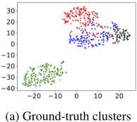
Figure 3: Treatment clusters in the synthetic dataset.
model each treatment separately, thus cannot capture the dependency among treatments. BART is limited in the strong ignorability assumption. Deconf-l and Deconf-q may capture latent confounders by utilizing the assignment of multiple treamtents, but they do not utilize the observed outcome, and also lack disentanglement, which is also the limitation of DIRECT-ND. We attribute the superiority of DIRECT to two key factors: (1) our framework leverages the multiple treatment assignment and observed outcome to capture more latent confounders; (2) the disentangled representation often leads to higher performance, which is in line with the conclusion in [Ma et al., 2019].
Generalization for New Treatments. We assess how the proposed framework can be generalized to predict the effects of treatments that are unseen in the training data. Since none of the baseline methods can handle unseen treatments, in each dataset, we randomly hold out 20% treatments and compare the performance of our framework in predicting the causal effect of the treatment assignment over the held out treatments with/without their assignment data. The results in Table 3 show that our model can achieve comparable performance for new treatments without retraining, which benefits from the trainable network for treatment representation learning.
4.4 Disentanglement & Interpretability
We visualize the treatment representation and color them w.r.t. their true/predicted clusters in Fig. 3. We observe that the predicted clusters are very close to the ground-truth. As the treatments' representation is aligned with the confounders' representation, it indicates good macro-level disentanglement of the representations of confounders. Due to
6
5
4
3
0.6 0.7 0.8
Level of disentanglement
(b) Amazon-3C
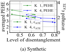
Figure 4: MTE estimation performance w.r.t. different levels of disentanglement of the representations of confounders.
space limit, we only show the results in the synthetic dataset, but the observations are similar in other datasets.
To investigate the relation between the disentanglement of confounders' representations and the MTE estimation performance, we vary the hyperparameter K and β to control the level of disentanglement, and Fig. 4 shows how the estimation performance varies w.r.t. different levels of disentanglement of the confounders' representations. Here the level of disentanglement of representation with dimension d is calculated by 1 - 2 d(d-1) ∑i,j |corr(i, j)|, where corr(i, j) is the correlation between dimension i and j. Due to space limit, we only show the results on datasets Synthetic and Amazon-3C, but similar observations can be found on the other dataset. As shown in Fig. 4, treatment clustering (K > 1) benefits the disentanglement, and higher levels of disentanglement often leads to better MTE estimation performance.
To further show the interpretability of the learned disentangled representations, we investigate their semantics in microlevel. On Amazon-3C, after training, we use a similar way to evaluate the micro-level disentanglement as [Ma et al., 2019; Wang et al., 2020]. We modify one dimension of the learned confounder representations by multiplying it with a temperature factor τ = 10, while keep all other dimensions fixed. Then we list the treatments with the biggest changes w.r.t. the predicted treatment assignment after modification in Table 4. Generally, we have two observations: 1) the treatments that are significantly affected can match the cluster of the modified dimension. This indicates a high-level interpretation, e.g., when we modify a dimension in z(k) , most of the top influenced treatments are about the musical instruments. This may imply that the cluster k corresponds to latent attributes related to musical instrument products; 2) most of the top influenced treatments contain a common word or semantically related words, which indicates that the model can capture the fine-grained latent factors by disentangled representation, e.g., when we modify a dimension, the top influenced treatments share the word "tune", which provides human-understandable semantics for the modified dimension.
5 RelatedWork
Multiple Treatment Effect Estimation. Traditional methods for the single cause can be extended to the multi-cause setting [Lopez et al., 2017; Zanutto et al., 2005; Lechner, 2001], and recent work [Sharma et al., 2020] applies the neural network. However, these works are still based on the
averaged PEHE
4
3
2
averaged ATE
| Manipulated dimension | Top-5 treatments | ||||
|---|---|---|---|---|---|
| In Cluster 1 | tune musician capo | tune tuner recording | loud tune bass | tune bass price | finger player tune |
| In Cluster 2 | size sizing width | long size old | longer little classic | sizing felt price | size longer feel |
| In Cluster 3 | battery charge phone | long battery old | headphone battery quick | light charger cost | access connect battery |
strong ignorability assumption. To mitigate this problem, a relaxed assumption called single strong ignorability is proposed in [Wang and Blei, 2019] for the multi-cause scenarios, which assumes that there do not exist unobserved singlecause confounders that causally affect the outcome and only one of the treatments. Despite its success in applications such as recommender systems [Wang et al., 2018] and medication analysis [Zhang et al., 2019], their captured latent confounders might be highly entangled and hard to interpret.
Disentangled Representation Learning. Disentangled representation learning has attracted significant attention recently. [Ma et al., 2019] introduces a macro-micro disentangled representation learning framework for recommender systems, which achieves macro disentanglement by inferring high-level user intentions and micro disentanglement to force each dimension capture an isolated factor. We use a similar way of hierarchical disentanglement but focus on the causal inference domain. In causal inference, a line of work [Hassanpour and Greiner, 2019; Zhang et al., 2020] identifies disentangled representations to separate the latent factors which influence the treatment assignment, the outcome, or both of them. Our work differs from them as the disentanglement in our work focuses on the confounders mixed in hierarchical patterns.
6 Conclusion
In this paper, we study a novel problem of disentangled multiple treatment effect estimation, and analyze its importance and challenges. We develop a novel framework DIRECT to learn disentangled representations of latent confounders for MTE estimation. Specifically, we improve the interpretability of the learned representations of confounders at both macro level and micro level. Then, we learn a trainable function to obtain the representation for each treatment by leveraging their inherent dependencies, which can be further generalized to unseen treatments. We conduct extensive experiments on different datasets, and the experimental results validate the effectiveness and interpretability of our proposed framework.
Acknowledgements
This material is, in part, supported by the National Science Foundation (NSF) under grants #2006844 and #1938167.
@inproceedings{ijcai2021p384,
  title     = {Multi-Cause Effect Estimation with Disentangled Confounder Representation},
  author    = {Ma, Jing and Guo, Ruocheng and Zhang, Aidong and Li, Jundong},
  booktitle = {Proceedings of the Thirtieth International Joint Conference on
               Artificial Intelligence, {IJCAI-21}},
  publisher = {International Joint Conferences on Artificial Intelligence Organization},
  editor    = {Zhi-Hua Zhou},
  pages     = {2790--2796},
  year      = {2021},
  month     = {8},
  note      = {Main Track},
  doi       = {10.24963/ijcai.2021/384},
  url       = {https://doi.org/10.24963/ijcai.2021/384},
}
TY - CPAPER TI - Multi-Cause Effect Estimation with Disentangled Confounder Representation AU - Ma, Jing AU - Guo, Ruocheng AU - Zhang, Aidong AU - Li, Jundong T2 - Proceedings of the Thirtieth International Joint Conference on Artificial Intelligence, IJCAI-21 PB - International Joint Conferences on Artificial Intelligence Organization PY - 2021 SP - 2790 EP - 2796 DO - 10.24963/ijcai.2021/384 UR - https://doi.org/10.24963/ijcai.2021/384 ER -Copied
Machine-readable versions of this paper, for tools and AI agents:





