
Residential Electric Load Forecasting via Attentive Transfer of Graph Neural Networks
Proceedings of the Thirtieth International Joint Conference on Artificial Intelligence. Main Track. Pages 2716-2722.
https://doi.org/10.24963/ijcai.2021/374
Keywords
- Machine Learning: Time-series; Data Streams
- Multidisciplinary Topics and Applications: Computational Sustainability
- Multidisciplinary Topics and Applications: Natural Sciences
Abstract
An accurate short-term electric load forecasting is critical for modern electric power systems' safe and economical operation.
Electric load forecasting can be formulated as a multi-variate time series problem. Residential houses in the same neighborhood may be affected by similar factors and share some latent spatial dependencies. However, most of the existing works on electric load forecasting fail to explore such dependencies. In recent years, graph neural networks (GNNs) have shown impressive success in modeling such dependencies. However, such GNN based models usually would require a large amount of training data. We may have a minimal amount of data available to train a reliable forecasting model for houses in a new neighborhood area. At the same time, we may have a large amount of historical data collected from other houses that can be leveraged to improve the new neighborhood's prediction performance. In this paper, we propose an attentive transfer learning-based GNN model that can utilize the learned prior knowledge to improve the learning process in a new area. The transfer process is achieved by an attention network, which generically avoids negative transfer by leveraging knowledge from multiple sources.
Extensive experiments have been conducted on real-world data sets. Results have shown that the proposed framework can consistently outperform baseline models in different areas.
- [Bahdanau et al., 2014] Dzmitry Bahdanau, Kyunghyun Cho, and Yoshua Bengio. Neural machine translation by jointly learning to align and translate. arXiv preprint arXiv:1409.0473, 2014.
- [Bräm et al., 2019] Timo Bräm, Gino Brunner, Oliver Richter, and Roger Wattenhofer. Attentive multi-task deep reinforcement learning. In Joint European Confer- ence on Machine Learning and Knowledge Discovery in Databases, pages 134-149. Springer, 2019.
- [Carreno et al., 2010] Edgar Manuel Carreno, Rodrigo Mazo Rocha, and Antonio Padilha-Feltrin. A cellular automaton approach to spatial electric load forecasting. IEEE Trans- actions on Power Systems, 26(2):532-540, 2010.
- [Corizzo et al., 2021] Roberto Corizzo, Michelangelo Ceci, Hadi Fanaee-T, and Joao Gama. Multi-aspect renewable energy forecasting. Information Sciences, 546:701-722, 2021.
- [Huang et al., 2005] Chao-Ming Huang, Chi-Jen Huang, and Ming-Li Wang. A particle swarm optimization to identify- ing the armax model for short-term load forecasting. IEEE Transactions on Power Systems, 20(2):1126-1133, 2005.
- [Kavousi-Fard et al., 2014] Abdollah Kavousi-Fard, Haidar Samet, and Fatemeh Marzbani. A new hybrid modified firefly algorithm and support vector regression model for accurate short term load forecasting. Expert systems with applications, 41(13):6047-6056, 2014.
- [Khodayar and Wang, 2018] Mahdi Khodayar and Jianhui Wang. Spatio-temporal graph deep neural network for short-term wind speed forecasting. IEEE Transactions on Sustainable Energy, 10(2):670-681, 2018.
- [Kong et al., 2017] Weicong Kong, Zhao Yang Dong, Youwei Jia, David J Hill, Yan Xu, and Yuan Zhang. Short-term residential load forecasting based on lstm re- current neural network. IEEE Transactions on Smart Grid, 10(1):841-851, 2017.
- [Li et al., 2017] Yaguang Li, Rose Yu, Cyrus Shahabi, and Yan Liu. Diffusion convolutional recurrent neural net- work: Data-driven traffic forecasting. arXiv preprint arXiv:1707.01926, 2017.
- [Malki et al., 2004] Heidar A Malki, Nicolaos B Karayian- nis, and Mahesh Balasubramanian. Short-term elec- tric power load forecasting using feedforward neural net- works. Expert Systems, 21(3):157-167, 2004.
- [Pan and Yang, 2009] Sinno Jialin Pan and Qiang Yang. A survey on transfer learning. IEEE Transactions on knowl- edge and data engineering, 22(10):1345-1359, 2009.
- [Papalexopoulos and Hesterberg, 1990] Alex D Papalex- opoulos and Timothy C Hesterberg. A regression-based approach to short-term system load forecasting. IEEE Transactions on Power Systems, 5(4):1535-1547, 1990.
- [Rajendran et al., 2015] Janarthanan Rajendran, Aravind S Lakshminarayanan, Mitesh M Khapra, P Prasanna, and Balaraman Ravindran. Attend, adapt and transfer: At- tentive deep architecture for adaptive transfer from mul- tiple sources in the same domain. arXiv preprint arXiv:1510.02879, 2015.
- [Tascikaraoglu, 2018] Akin Tascikaraoglu. Evaluation of spatio-temporal forecasting methods in various smart city applications. Renewable and Sustainable Energy Reviews, 82:424-435, 2018.
- [Vilalta and Drissi, 2002] Ricardo Vilalta and Youssef Drissi. A perspective view and survey of meta-learning. Artificial intelligence review, 18(2):77-95, 2002.
- [Weiss et al., 2016] Karl Weiss, Taghi M Khoshgoftaar, and DingDing Wang. A survey of transfer learning. Journal of Big data, 3(1):9, 2016.
- [Wu et al., 2014] Di Wu, Haibo Zeng, and Benoit Boulet. Neighborhood level network aware electric vehicle charg- ing management with mixed control strategy. In 2014 IEEE International Electric Vehicle Conference (IEVC), pages 1-7. IEEE, 2014.
- [Wu et al., 2017] Di Wu, Boyu Wang, Doina Precup, and Benoit Boulet. Boosting based multiple kernel learn- ing and transfer regression for electricity load forecast- ing. In Joint European Conference on Machine Learn- ing and Knowledge Discovery in Databases, pages 39-51. Springer, 2017.
- [Wu et al., 2019a] Di Wu, Boyu Wang, Doina Precup, and Benoit Boulet. Multiple kernel learning-based transfer re- gression for electric load forecasting. IEEE Transactions on Smart Grid, 11(2):1183-1192, 2019.
- [Wu et al., 2019b] Zonghan Wu, Shirui Pan, Guodong Long, Jing Jiang, and Chengqi Zhang. Graph wavenet for deep spatial-temporal graph modeling. arXiv preprint arXiv:1906.00121, 2019. IJCAI
- [Wu et al., 2020] Zonghan Wu, Shirui Pan, Guodong Long, Jing Jiang, Xiaojun Chang, and Chengqi Zhang. Con- necting the dots: Multivariate time series forecasting with graph neural networks. arXiv preprint arXiv:2005.11650, 2020.
- [Yu et al., 2017] Bing Yu, Haoteng Yin, and Zhanxing Zhu. Spatio-temporal graph convolutional networks: A deep learning framework for traffic forecasting. arXiv preprint arXiv:1709.04875, 2017. IJCAI
- [Zhou et al., 2018] Jie Zhou, Ganqu Cui, Zhengyan Zhang, Cheng Yang, Zhiyuan Liu, Lifeng Wang, Changcheng Li, and Maosong Sun. Graph neural networks: A review of methods and applications. arXiv preprint arXiv:1812.08434, 2018.
References were extracted automatically from the PDF and may contain errors.
Full text extracted automatically from the PDF; figures, tables and equations may differ. The PDF is the version of record.
1 Introduction
Electric load forecasting is of significant importance for the efficient operation of modern power grids. An accurate electric load forecasting is beneficial to the controlling and planning the operation of modern electric grid systems. Based on the time horizon, electric load forecasting can range from short-term (minutes or hours ahead) to long-term forecasting (years ahead). Among them, short-term load forecasting (STLF) is mainly used to assist real-time energy dispatching in the practice [Wu et al., 2014], and thus it is of great interest in the industry. However, an accurate STLF is increasingly difficult to achieve nowadays because the modern power system has been become more and more sophisticated. On the one hand, a variety of electric applicants have been adopted in the power network. On the other hand, a fast-growing amount of renewable sources have been adopted for the power generation side. Renewable energy sources, such as solar energy and wind energy generations, are desirable for sustainable development. However, compared to traditional energy sources, they are sensitive to weather conditions and have high volatility outputs.
Factors related to STLF include temperature, humidity, electronic appliances usage in a household, and so forth. These uncertain factors hinder the accuracy of an STLF model. Different types of approaches have been investigated to improve the accuracy of STLF. As a typical timeseries regression problem, STLF can be tackled by classic methods such as multivariate linear regression [Papalexopoulos and Hesterberg, 1990], and autoregressive moving average with exogenous variable [Huang et al., 2005]. Besides classic methods, machine learning-based methods have also been gaining attention for solving STLF in recent years because machine learning methods are more capable of capturing complex nonlinear relationships [Wu et al., 2019a]. For instance, various machine learning models have been reported for STLF, including support vector regression (SVR) [Kavousi-Fard et al., 2014], kernel-based method [Wu et al., 2017], and feed-forward neural network (FNN) [Malki et al., 2004]. Recurrent neural networks (RNNs) and their variants, such as long short-term memory (LSTM) and gated recurrent unit (GRU), are found promising in solving sequence problems [Kong et al., 2017].
However, the aforementioned methods only utilize historical temporal values from electric load and weather information. Besides using the temporal values, researchers are also paying attention to investigate the spatial correlation between different units [Carreno et al., 2010; Corizzo et al., 2021], as the spatial correlation can be utilized to improve the prediction accuracy. In terms of spatial correlation between residential households, researchers have also built models that can extract spatial information (i.e., the relation between households) in an electric grid to improve the accuracy of STLF [Tascikaraoglu, 2018]. Load forecasting using spatial correlations is usually referred to as spatial-temporal STLF. Spatialtemporal STLF is based on the hypothesis that load consumption patterns between households might share similar trends [Tascikaraoglu, 2018].
Besides electricity data, the latent dependencies between units have also been utilized for other time-series problems such as traffic prediction and wind prediction. Graph neural network (GNN) has demonstrated its effectiveness on these problems. For instance, GNN based models have demonstrated impressive success in traffic prediction [Wu et al., 2020; Wu et al., 2019b; Li et al., 2017; Yu et al., 2017] and wind speed prediction [Khodayar and Wang, 2018]. However, GNN-based spatial-temporal models have been rarely studied for STLF problems. Since GNN has demonstrated its capability of capturing latent dependencies for time series problems, in this paper, we propose to use GNN for shortterm load forecasting.
In the real world, we may not be able to have enough data to learn a reliable machine learning forecasting model. Transfer learning can be used to deal with such challenges. A multi-kernel based transfer learning algorithm has been proposed to transfer knowledge learned from source domains (e.g., data-sufficient domains) to the target domain (e.g., the domain we are interested in but with a limited amount of data) [Wu et al., 2019a]. However, to the best of our knowledge, a transfer learning framework for GNN has not yet been well studied for time series problems, especially STLF. The goal of this paper is to use GNN and transfer learning on STLF for domains where we do not have a large amount of data. Specifically, we propose a transfer learning framework to transfer the spatial-temporal knowledge learned by GNN-based models from source domains to the target domain. Therefore, this framework not only transfers the knowledge from the historical temporal data but also transfers the knowledge of latent dependencies learned by the GNN-based model.
2 Technical Background
2.1 GNN basedModel for Time-Series Regression
GNN has been developed into many variants and becoming popular in recent years [Zhou et al., 2018]. It has demonstrated its excellence in exploiting non-Euclidean spatial relationships to improve the prediction accuracy for different time-series forecasting problems [Wu et al., 2019b; Wu et al., 2020]. To utilize GNN-based models, data has to be presented in the form of graph structure G = (V, E), where vi ∈ V represents a node and eij ∈ E denotes an edge pointing from vi to vj. In the meanwhile, an adjacency matrix A ∈ Rn×n is used to quantitatively describe the connectedness between nodes, i.e. Aij = 1 if eij ∈ E and Aij = 0 if eij ̸∈ E. To extract the spatial information in graph structure data, graph convolutions are the most common approaches. Methods for graph convolutions are categorized into spatial-based and spectral-based [Zhou et al., 2018]. To illustrate how graph convolution extracts spatial information, the diffusion convolution neural network, which is one of the spatial-based graph convolution methods [Li et al., 2017; Wu et al., 2019b], will be introduced here. This method regards graph convolution as a diffusion process, in which information is transmitted between nodes connected with a possibility transition matrix calculated according to the adjacency matrix. The diffusion graph convolution is defined as
where ∗ is the element-wise product, P = A/rowsum(A) is the possibility transition matrix, X is the graph structure input data, Hk is the hidden output of the kth diffusion step, Wk is the learnable parameters for the kth diffusion step, and Z is the final output of a diffusion graph convolution layer. By combining graph convolution and spatial-temporal time-series input data, GNN-based models can solve spatialtemporal time-series regression problems [Wu et al., 2020].
2.2 Residential Houses based Graph Structure for STLF
Spatial-temporal STLF can be regarded as a spatial-temporal time series prediction problem. Given the historical values of a group of households, the model aims at learning from the temporal data and spatial relationships in order to predict the load values ahead. Mathematically, Xt = {xt1 , ..., xtn } represent the load values at the t-th time step for households 1, 2, ..., n. A spatial-temporal electric load dataset is represented by {X1 , ...,X T } ∈ Rn×T , with total house number n and a total time step of T. Then, by combining the spatial-temporal dataset and the adjacency matrix that describes the correlation between households, a graph structure data {X1 , ...,X T ,A} is formulated, where XT ∈ Rn consists of the load values of n households at the time step of T , and A ∈ Rn×n is the adjacency matrix. The graph structure will facilitate the operation of GNN for STLF.
2.3 Transfer Learning
Machine learning based STLF methods, especially deep learning based methods would require a sufficient amount of data to achieve reasonable accuracy. However, data collection could be expensive and difficult in practice, especially for an STLF model to be applied in a new-built smart grid system. The concept of transfer learning is designed to tackle this kind of problem [Pan and Yang, 2009]. In transfer learning, the domain we are interested in refers to the target domain, usually lacking data. Meanwhile, sufficient data might be available in other related domains. These related domains refer to source domains. Therefore, it is reasonable and desirable to transfer knowledge learned from source domains to the target domain so that a better generalization can be achieved in the target domain even with a relatively small amount of data. Besides designing a mechanism to transfer knowledge, a challenge in transferring knowledge is negative transfer [Weiss et al., 2016], which deteriorates the complete model when the target domain and source domains are not closely related. Thus, it is necessary to distinguish and exclude knowledge from certain source domains that might hinder the learning in the target domain. Different types of meta-learning methods [Vilalta and Drissi, 2002] have been proposed to enable the models to learn fast. However, most of these methods require that the learning tasks should be sampled from the same task distribution. Therefore these methods are not suitable for our problem.
3 Methodology
To solve the problem of negative transfer generically, an attentive and adaptive transfer architecture has been proposed for reinforcement learning [Rajendran et al., 2015]. This architecture's key contribution is that an attention mechanism based on a deep neural network learns to assign weights to pre-learned solutions so that the most suitable solutions are decided to be transferred. A similar architecture of attentionbased ensemble has been also reported in [Br¨am et al., 2019], in which an attention network learns to group task knowledge into sub-networks on a state-level granularity.
Inspired by the attentive and adaptive transfer learning applied in reinforcement learning [Rajendran et al., 2015; Br¨am et al., 2019], we propose an attentive transfer framework for transferring knowledge from GNN models trained in source domains. These GNN models in source domains, as indicated by Wu et al [Wu et al., 2020], have learned not only temporal knowledge but also the knowledge of latent spatial dependencies.
Therefore, it is expected that a transfer learning framework for GNN models can transfer both the temporal and spatial knowledge in trained GNN models. Also, this framework hypothesizes that as the spatial information explored by a GNN-based model can improve the accuracy of the STLF in a source domain, spatial knowledge learned from source domains can also be exploited to improve a transfer learning framework. In this section, the formation of STFL based on graph structure will be given first. The attentive transfer framework will be illustrated afterward.
3.1 STLF based on Graph Structure
As demonstrated in Sec.2.2, a graph structure data {X1 , ...,X T ,A} consists of the historical load data of every household and the adjacency matrix describing the correlation between households. This graph structure data can be operated by a GNN-based STLF model f(·), which aims to learn from the Graph structure data of last h time steps to predict the spatial-temporal data of the next time step, i.e. {Xt-h+1 , ...,X t ,A} f(·) -→ Xt+1 . In addition, the correlations between households are related to locations, living habits, types of appliances, and so forth. Thus, the adjacency matrix A for STLF is difficult to predetermine. So, the GNN model that can discover latent correlation, such as [Wu et al., 2019b], can be preferable for spatial-temporal STLF.
3.2 Proposed Forecasting Framework
Figure 1 illustrates the transfer learning framework based on a set of base GNN models. This framework consists of three parts: a base GNN network learned from the target domain, N GNN models learned from source domains, and an attention network learning to assign weights. The base GNN model is trained with insufficient data in the training set of the target domain. The N source GNN models are pre-trained by a sufficient amount of data in the corresponding source domains. The base model yields the base output ˆ yBase and the N source models yield source outputs ˆ ysrc,1, ˆ ysrc,2, ..., ˆ ysrc,N. It is noted that all GNNmodels share the same node number so that they can be merged afterward.
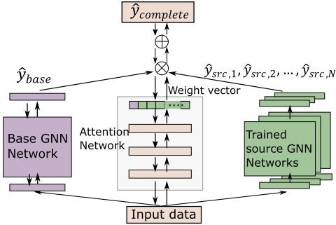
The attention network is designed to learn to weight the models' outputs ˆ ysrc,1, ˆ ysrc,2, ..., ˆ ysrc,N and ˆ yBase. The attention network is based on a multi-layer perceptron (MLP), which can be represented as (e1,X, .., eN+1,X) = fa(X; θa), where X is the input data, θa is learnable parameters, (e1,X, .., eN+1,X) are outputs with the dimension of RN+1 . The output from the MLP is converted to weights assigned to models by the soft-attention mechanism, which allows the attention network to generate more than one non-zero weight [Rajendran et al., 2015; Bahdanau et al., 2014]
where ∑N+1 i=1 wi = 1,wi ∈ [0, 1]. Therefore, the complete model's output ˆ ycomplete is the weighted summation of the outputs from source models and the base model
Different approaches are adopted to update parameters in source models, the base model, and the attention network. All source models are pre-trained and their parameters are kept constant during the attentive ensemble. Parameters in the base model are updated according to the loss calculated by the output of the complete model ˆ yBase and the real value in the data of target domain yreal, i.e. LT (ˆ yBase, yreal). Parameters in the attention network are updated according to the final output from the complete model ˆ ycomplete and the real value in the data of target domain yreal, i.e., LT (ˆ ycomplete, yreal). As indicated in Figure 1, there are two separate back-propagations in the base GNN network and in the attention network. The loss function is selected as the mean absolute error function
where n is the total household number.
4 Experiment
This framework will be evaluated upon the dataset OpenEI 1 . The dataset consists of residential hourly electric load data recorded in different cities in the year 2012. Specifically, 8760 hourly data points are in the record for each house.
4.1 Experiment Setup
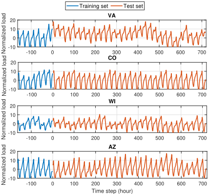
In this section, experiments are conducted to transfer knowledge from six source domains to four target domains. The six source domains contain source data from Pennsylvania (PA), New Mexico (NM), New York (NY), Oregon (OR), Alabama (AL), and Texas (TX), respectively. For convenience, these six source domains are denoted as source domains 1 to 6, respectively. Each source data consists of 10 households' historical temporal electric loads in the first 90 days of the year (2160 data-points). A source model is trained with the corresponding dataset. All source data is divided into training/validation/test sets with a ratio of 0.7/0.2/0.1 chronologically. In addition, Graph WaveNet [Wu et al., 2019b] is the chosen model as an example to validate the attentive ensemble framework. The reason is that Graph WaveNet has the ability to discover the relationship between nodes in a graph without any prerequisite knowledge of nodes relationships. This ability to discover hidden node relations makes Graph WaveNet a potential candidate for spatio-temporal STLF. All source models are Graph WaveNets with the same set of parameters listed in Table 1. This set of hyperparameters is the same as the one in [Wu et al., 2019b] which also demonstrates a good performance on the OpenEI dataset. All source models are pre-trained individually and kept fixed during the subsequent training in the attentive ensemble framework. It is noted that source models are trained to predict the onehour load values of all households ˆ y ∈ RN , with the input of the latest 4 time-steps historical temporal load values of all households X ∈ RN×T , where household number N = 10 and time step T = 4. The four target domains include target data from Virginia (VA), Colorado (CO), Wisconsin (WI), and Arizona (AZ), respectively. Each target data has 10 households' temporal load values of 37 days (888 datapoints) between January and February. The target data is divided into training/test sets with a ratio of 7/30 chronologically. All data in the source or target domain is normalized by the mean value µtrain and the standard deviation σtrain of the training set in the corresponding domain. Figure 2 shows the aggregated normalized load profiles in different target areas. The normalized load patterns in AZ and CO are more regular than the patterns in VA and WI.
1 available at https://openei.org/datasets/files/961/pub/ RESIDENTIALLOADDATAEPLUSOUTPUT/HIGH/
In the attentive ensemble framework, the base model is a Graph WaveNet with the same parameters in Table 1 except the batch size and epoch number. The attention network consists of a flatten layer followed by a three-layer perceptron with hidden layer sizes of (32, 32). During the training for the complete model, the batch size is 8 and the epoch number is 100. The complete model was implemented using PyTorch library on a desktop with a NVIDIA GeForce GTX 1080Ti graphics processing unit card and 32 GB memory.
As illustrated in Figure 1, the attentive ensemble framework updates the parameters in the base model and the parameters in the attention network separately. After the training, besides the complete model obtained by the attentive ensemble, a base model trained by the target training set is also obtained. To demonstrate how the attention network transfers knowledge from domains, the complete model, base model, and the 6 source models will be compared and evaluated by the data in the target test set. Also, the aforementioned models are compared with baselines including linear regression (Regr), feedforward neural networks (FNN) with hidden units of (32, 32), support vector regression (SVR), and a stacked LSTM with hidden units of (32, 32). These baselines are trained with the target training data.
Mean absolute percentage error (MAPE) and mean absolute error (MAE) are used as the metrics for evaluation: MAPE = | ˆ y-y y | × 100%, and MAE = |ˆ y - y|. In addition, similar to [Kong et al., 2017], the average error of individual loads and the error of aggregated load will be evaluated.
4.2 Experimental Result
Performance of Models
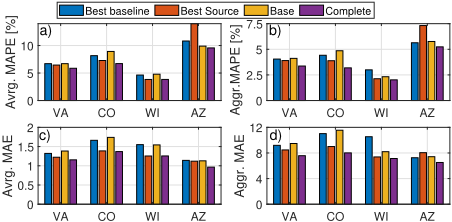
Table 2 demonstrates the performance of 6 source models, the base model, and the complete model on the test sets of the four different target domains. And Table 3 demonstrates the baselines' performance. Figure 3 visualizes the selected data presented in Table 2 and 3, and it compares the performance of the best baseline, the best source model, the base models and the complete model in different target areas under different evaluation metrics.
| Name | Value |
|---|---|
| Sequence of dilation factor | (1,2,1,2,1,2,1,2) |
| Layer of GWN | 8 |
| Size of node embeddings | 10 |
| Diffusion step | 4 |
| Drop-out rate | 0.3 |
| Learning rate | 0.001 |
| Batch size | 128 |
| Epoch number | 120 |
Also, to intuitively understand the performance improvement when comparing different models with the best baselines in different target areas, Figure 4 presents the error improvement percentage from the best baselines to the selected models. The best source model evidently outperforms the best baseline in the target areas of VA, CO, and WI. But the best source model performs significantly worse than the baseline in the target area of AZ. This phenomenon shows that though trained with an abundant amount of source data, source models are still possibly incompetent in some target data. In terms of the base model, because it is trained by insufficient target data, its performance is hardly comparable with the best baselines in different target areas. Thus, VA
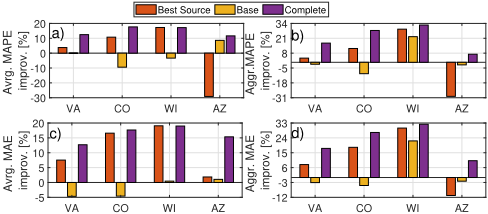
it is difficult to achieve accurate STLF with a single baseline/source/base model. And the complete model steadily and evidently excels the best baseline in all target areas and evaluation metrics. This shows that transfer learning is necessary in achieve accurate STLF when target data is insufficient.
From Table 2 and Figure 3, it is noticed that the target data from different areas significantly influences the performance of source models as well as the base model. When comparing the performance between source models, although source model 4 performs the best in all target areas under most of the evaluation metrics, source model 4 does not outperform the other source models by a large margin. Also, even with a limited amount of training data in the target domain, the base model is possible to be relatively well-trained and outperform source models. In Table 2, the base model performs significantly worse than the best source models in the area of VA, CO, and WI. But in the target area AZ, the base model outperforms all source models under all evaluation metrics except the average MAE of individual loads. Therefore, even though the best model varies among source models and the base model in different target areas, the attentive ensemble framework can always lead to a complete model with the performance equivalent with or better than the best source/base model. This excellent performance relies on the attention network, which successful ensembles the results from these models in an optimal way.
Impact of the Learned Weights
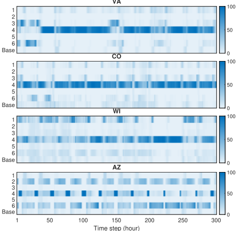
Figure 5 visualizes the weights of the attention network output in different target test sets. From the patterns, it is noticed that the weight changes with input data. This shows that the attention network recognizes the pattern of input data and assigns weights to corresponding suitable models. Also, the weight pattern varies evidently in different target test sets. In target areas of VA, CO, and WI, most of the weights are assigned to source model 4. However, in AZ, besides source model 4, source model 2 and 6 also demonstrate more evident and frequent participation during the ensemble, compared to the other target areas.
| Target Area | Metrics | SRC 1 | SRC 2 | SRC 3 | SRC 4 | SRC 5 | SRC 6 | Base | Complete |
|---|---|---|---|---|---|---|---|---|---|
| VA | Avrg. MAPE Aggr. MAPE Avrg. MAE Aggr. MAE | 6.98% 4.75% 1.36 10.98 | 7.04% 4.61% 1.34 9.88 | 6.82% 4.28% 1.24 9.27 | 6.64% 3.90% 1.22 8.47 | 6.45% 4.16% 1.26 9.15 | 6.85% 4.02% 1.32 8.76 | 6.70% 4.11% 1.38 9.48 | 5.87% 3.37% 1.15 7.57 |
| CO | Avrg. MAPE Aggr. MAPE Avrg. MAE Aggr. MAE | 7.80% 4.66% 1.52 11.00 | 7.74% 3.88% 1.52 9.32 | 7.83% 4.77% 1.52 11.14 | 7.28% 3.90% 1.39 9.00 | 8.87% 3.95% 1.57 9.72 | 10.14% 4.37% 1.70 10.34 | 8.93% 4.86% 1.74 11.55 | 6.72% 3.19% 1.37 8.01 |
| WI | Avrg. MAPE Aggr. MAPE Avrg. MAE Aggr. MAE | 4.08% 2.55% 1.34 9.01 | 5.15% 3.26% 1.61 11.12 | 4.23% 2.71% 1.36 9.38 | 3.83% 2.13% 1.25 7.38 | 5.22% 3.01% 1.58 10.48 | 5.89% 3.27% 1.78 11.30 | 4.79% 2.32% 1.54 8.20 | 3.84% 2.02% 1.26 7.14 |
| AZ | Avrg. MAPE Aggr. MAPE Avrg. MAE Aggr. MAE | 15.13% 8.93% 1.32 10.93 | 16.46% 9.63% 1.23 9.31 | 15.30% 9.42% 1.24 10.49 | 13.98% 7.31% 1.12 8.04 | 15.44% 9.22% 1.22 9.71 | 14.54% 8.58% 1.22 9.10 | 9.89% 5.76% 1.13 7.42 | 9.57% 5.24% 0.97 6.52 |
| Area | Metric | FNN | LSTM | Regr | SVR |
|---|---|---|---|---|---|
| VA Avrg. Aggr. Avrg. Aggr. | MAPE 9.17% MAPE 4.88% MAE 1.95 MAE 11.49 | 12.61% 9.06% 3.23 22.06 | 7.37% 4.15% 1.48 9.48 | 1.32 9.19 | 6.70% 4.05% |
| CO Avrg. MAPE Aggr. MAPE Avrg. MAE Aggr. MAE | 11.99% 5.31% 2.24 12.77 | 13.88% 6.10% 2.83 14.89 | 8.33% 4.42% 1.73 11.02 | 1.66 11.38 | 8.16% 4.62% |
| WI Avrg. MAPE Aggr. MAPE Avrg. MAE Aggr. MAE | 7.16% 3.84% 2.13 13.07 | 6.95% 3.67% 2.39 13.03 | 4.63% 2.99% 1.55 10.53 | 4.95% 3.36% 1.65 11.74 | |
| AZ Avrg. MAPE Aggr. MAPE Avrg. MAE Aggr. MAE | 10.82% 5.63% 1.17 7.25 | 12.07% 5.92% 1.30 7.84 | 12.04% 6.56% 1.16 | 8.07 | 11.69% 6.26% 1.14 7.97 |
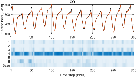
To unveil the relation between electric load profiles and the weight pattern, Figure 6 demonstrates the real aggregated load profile in the test set of CO, the predicted value by the complete model, and the corresponding weight pattern when calculating the predicted value. It is noticed that the attention network assigns most of the weight to the source model 4 along with the ascending parts of the load profile. During the descending parts of the load profile, the source model 4 has less weight assigned. In the meanwhile, the source model 1, 3, 6 and the base model increase their participation in the ensemble process.
In summary, the experimental results show that the proposed framework successfully achieves transfer knowledge from source GNN networks. The attention network also solves the problem of negative transfer by generically assigning weights to source models and the base model.
5 Conclusion
In conclusion, this paper proposes an attentive ensemble framework to solve the problem of insufficient training data in STLF via transfer learning. By learning an attention network to assign weights to source models and the base model, the proposed framework successfully integrates knowledge from source GNN networks as well as the base model. The concern on negative transfer has also been released generically by the attention network. Experiments have been conducted in four different areas. The experimental results show that the proposed method can outperform the baselines significantly and perform robustly in different areas. Furthermore, though Graph WaveNet is used as the GNN network in the experiments, the proposed framework can also integrate various kinds of GNN models. In the future, we plan to validate this framework on more problems with different GNN networks.
@inproceedings{ijcai2021p374,
  title     = {Residential Electric Load Forecasting via Attentive Transfer of Graph Neural Networks},
  author    = {Lin, Weixuan and Wu, Di},
  booktitle = {Proceedings of the Thirtieth International Joint Conference on
               Artificial Intelligence, {IJCAI-21}},
  publisher = {International Joint Conferences on Artificial Intelligence Organization},
  editor    = {Prof. Zhi-Hua Zhou},
  pages     = {2716--2722},
  year      = {2021},
  month     = {8},
  note      = {Main Track},
  doi       = {10.24963/ijcai.2021/374},
  url       = {https://doi.org/10.24963/ijcai.2021/374},
}
TY - CPAPER TI - Residential Electric Load Forecasting via Attentive Transfer of Graph Neural Networks AU - Lin, Weixuan AU - Wu, Di T2 - Proceedings of the Thirtieth International Joint Conference on Artificial Intelligence, IJCAI-21 PB - International Joint Conferences on Artificial Intelligence Organization PY - 2021 SP - 2716 EP - 2722 DO - 10.24963/ijcai.2021/374 UR - https://doi.org/10.24963/ijcai.2021/374 ER -Copied
Machine-readable versions of this paper, for tools and AI agents:





