
Towards Understanding Deep Learning from Noisy Labels with Small-Loss Criterion
Proceedings of the Thirtieth International Joint Conference on Artificial Intelligence. Main Track. Pages 2469-2475.
https://doi.org/10.24963/ijcai.2021/340
Keywords
- Machine Learning: Learning Theory
- Machine Learning: Deep Learning
- Machine Learning: Classification
- Machine Learning: Weakly Supervised Learning
Abstract
Deep neural networks need large amounts of labeled data to achieve good performance. In real-world applications, labels are usually collected from non-experts such as crowdsourcing to save cost and thus are noisy. In the past few years, deep learning methods for dealing with noisy labels have been developed, many of which are based on the small-loss criterion. However, there are few theoretical analyses to explain why these methods could learn well from noisy labels. In this paper, we theoretically explain why the widely-used small-loss criterion works. Based on the explanation, we reformalize the vanilla small-loss criterion to better tackle noisy labels. The experimental results verify our theoretical explanation and also demonstrate the effectiveness of the reformalization.
- [Algan and Ulusoy, 2019] Görkem Algan and Ilkay Ulusoy. Image classification with deep learning in the presence of noisy labels: A survey. arXiv, 2019.
- [Arazo et al., 2019] Eric Arazo, Diego Ortego, Paul Albert, Noel O'Connor, and Kevin Mcguinness. Unsupervised label noise modeling and loss correction. In ICML, 2019.
- [Arpit et al., 2017] Devansh Arpit, Stanislaw Jastrzkebski, Nicolas Ballas, David Krueger, Emmanuel Bengio, Maxinder S Kanwal, Tegan Maharaj, Asja Fischer, et al. A closer look at memorization in deep networks. In ICML, 2017.
- [Berthelot et al., 2019] David Berthelot, Nicholas Carlini, Ian Goodfellow, Nicolas Papernot, Avital Oliver, et al. Mixmatch: A holistic approach to semi-supervised learning. In NIPS, 2019.
- [Chen et al., 2019] Pengfei Chen, Ben Ben Liao, Guangyong Chen, and Shengyu Zhang. Understanding and utilizing deep neural networks trained with noisy labels. In ICML, 2019.
- [Deng et al., 2009] Jia Deng, Wei Dong, Richard Socher, Li-Jia Li, Kai Li, and Li Fei-Fei. Imagenet: A large-scale hierarchical im- age database. In CVPR, 2009.
- [Ghosh et al., 2017] Aritra Ghosh, Himanshu Kumar, and P. S. Sas- try. Robust loss functions under label noise for deep neural net- works. In AAAI, 2017.
- [Goldberger and Ben-Reuven, 2017] Jacob Goldberger and Ehud Ben-Reuven. Training deep neural-networks using a noise adap- tation layer. In ICLR, 2017.
- [Han et al., 2018a] Bo Han, Jiangchao Yao, Gang Niu, Mingyuan Zhou, Ivor W. Tsang, Ya Zhang, and Masashi Sugiyama. Mask- ing: A new perspective of noisy supervision. In NIPS, 2018.
- [Han et al., 2018b] Bo Han, Quanming Yao, Xingrui Yu, Gang Niu, Miao Xu, Weihua Hu, Ivor W. Tsang, and Masashi Sugiyama. Co-teaching: Robust training of deep neural networks with ex- tremely noisy labels. In NIPS, 2018.
- [Hendrycks et al., 2018] Dan Hendrycks, Mantas Mazeika, Duncan Wilson, and Kevin Gimpel. Using trusted data to train deep net- works on labels corrupted by severe noise. In NIPS, 2018.
- [Hu et al., 2020] Wei Hu, Zhiyuan Li, and Dingli Yu. Simple and effective regularization methods for training on noisily labeled data with generalization guarantee. In ICLR, 2020.
- [Jiang et al., 2018] Lu Jiang, Zhengyuan Zhou, Thomas Leung, Li- Jia Li, et al. Mentornet: Learning data-driven curriculum for very deep neural networks on corrupted labels. In ICML, 2018.
- [Jiang et al., 2020] Lu Jiang, Di Huang, Mason Liu, and Weilong Yang. Beyond synthetic noise: Deep learning on controlled noisy labels. In ICML, 2020.
- [Li et al., 2017] Wen Li, Limin Wang, Wei Li, Eirikur Agustsson, and Luc V. Gool. Webvision database: Visual learning and un- derstanding from web data. arXiv, 2017.
- [Li et al., 2020] Mingchen Li, Mahdi Soltanolkotabi, and Samet Oymak. Gradient descent with early stopping is provably ro- bust to label noise for overparameterized neural networks. In AISTATS, 2020.
- [Liu et al., 2020] Sheng Liu, Jonathan Niles-Weed, Narges Raza- vian, and Carlos Fernandez-Granda. Early-learning regulariza- tion prevents memorization of noisy labels. In NIPS, 2020.
- [Ma et al., 2018] Xingjun Ma, Yisen Wang, Michael E. Houle, Shuo Zhou, Sarah M. Erfani, Shu-Tao Xia, et al. Dimensionality- driven learning with noisy labels. In ICML, 2018.
- [Natarajan et al., 2013] Nagarajan Natarajan, Inderjit S. Dhillon, Pradeep K. Ravikumar, and Ambuj Tewari. Learning with noisy labels. In NIPS, 2013.
- [Patrini et al., 2017] Giorgio Patrini, Alessandro Rozza, Aditya K. Menon, Richard Nock, and Lizhen Qu. Making deep neu- ral networks robust to label noise: A loss correction approach. In CVPR, 2017.
- [Raykar et al., 2010] Vikas C. Raykar, Shipeng Yu, Linda H. Zhao, Gerardo H. Valadez, Charles Florin, Luca Bogoni, and Linda Moy. Learning from crowds. JMLR, 2010.
- [Rolnick et al., 2017] David Rolnick, Andreas Veit, Serge Be- longie, and Nir Shavit. Deep learning is robust to massive label noise. arXiv, 2017.
- [Shen and Sanghavi, 2019] Yanyao Shen and Sujay Sanghavi. Learning with bad training data via iterative trimmed loss min- imization. In ICML, 2019.
- [Song et al., 2019] Hwanjun Song, Minseok Kim, and Jae-Gil Lee. Selfie: Refurbishing unclean samples for robust deep learning. In ICML, 2019.
- [Sukhbaatar et al., 2014] Sainbayar Sukhbaatar, Joan Bruna, Manohar Paluri, Lubomir Bourdev, and Rob Fergus. Training convolutional networks with noisy labels. In ICLR workshop, 2014.
- [Tanaka et al., 2018] Daiki Tanaka, Daiki Ikami, Toshihiko Ya- masaki, and Kiyoharu Aizawa. Joint optimization framework for learning with noisy labels. In CVPR, 2018.
- [Wang et al., 2020] Zhuowei Wang, Jing Jiang, Bo Han, Lei Feng, Bo An, Gang Niu, and Guodong Long. Seminll: A framework of noisy-label learning by semi-supervised learning. arXiv, 2020.
- [Wei et al., 2020] Hongxin Wei, Lei Feng, Xiangyu Chen, and Bo An. Combating noisy labels by agreement: A joint training method with co-regularization. In CVPR, 2020.
- [Xia et al., 2019] Xiaobo Xia, Tongliang Liu, Nannan Wang, Bo Han, Chen Gong, Gang Niu, and Masashi Sugiyama. Are anchor points really indispensable in label-noise learning? In NIPS, 2019.
- [Xia et al., 2020] Xiaobo Xia, Tongliang Liu, Bo Han, Nannan Wang, Mingming Gong, Haifeng Liu, et al. Part-dependent label noise: Towards instance-dependent label noise. In NIPS, 2020.
- [Xu et al., 2019] Yilun Xu, Peng Cao, Yuqing Kong, and Yizhou Wang. L DMI: An information-theoretic noise-robust loss func- tion. In NIPS, 2019.
- [Yi and Wu, 2019] Kun Yi and Jianxin Wu. Probabilistic end-to- end noise correction for learning with noisy labels. In CVPR, 2019.
- [Yu et al., 2019] Xingrui Yu, Bo Han, Jiangchao Yao, Gang Niu, Ivor W. Tsang, and Masashi Sugiyama. How does disagreement help generalization against label corruption? In ICML, 2019.
- [Zhang and Sabuncu, 2018] Zhilu Zhang and Mert Sabuncu. Gen- eralized cross entropy loss for training deep neural networks with noisy labels. In NIPS, 2018.
- [Zhang et al., 2017] Chiyuan Zhang, Samy Bengio, Moritz Hardt, Benjamin Recht, and Oriol Vinyals. Understanding deep learning requires rethinking generalization. In ICLR, 2017.
References were extracted automatically from the PDF and may contain errors.
Full text extracted automatically from the PDF; figures, tables and equations may differ. The PDF is the version of record.
1 Introduction
Deep neural networks (DNNs) have achieved great success in many real-world applications, but rely on large-scale data with accurate labels [Deng et al., 2009]. Obtaining largescale accurate labels is expensive while the alternative methods such as crowdsourcing [Raykar et al., 2010] and web queries [Jiang et al., 2020] can easily provide extensive labeled data, but unavoidably incur noisy labels. The performance of deep neural networks may be severely hurt if these noisy labels are blindly used [Zhang et al., 2017], and thus how to learn with noisy labels has become a hot topic.
In the past few years, many deep learning methods for tackling noisy labels have been developed. Some methods try to exploit noise-robust loss functions, e.g., MAE loss [Ghosh et al., 2017], Truncated Lq loss [Zhang and Sabuncu, 2018] and the information-theoretic loss [Xu et al., 2019]. These methods do not consider the specific information about label noise, and thus usually have limited utility in real-world applications. Some methods use the transition matrix to model label noise and construct an unbiased loss term to alleviate the influence of noisy labels [Sukhbaatar et al., 2014; Patrini et al., 2017; Goldberger and Ben-Reuven, 2017; Han et al., 2018a; Hendrycks et al., 2018]. However, the performance of these methods is usually suboptimal due to the difficulty of accurately estimating the noise transition matrix. Some other methods try to correct the noisy labels [Ma et al., 2018; Arazo et al., 2019; Yi and Wu, 2019], but may suffer from the false correction. Sometimes, although correcting the noisy labels might be challenging especially for the classification task with a large number of classes, the detection of noisy labels is relatively easy. Along this direction, the sample selection strategy with the widely-used small-loss criterion has been proposed, i.e., treating the examples with small loss as the clean data and using them in the training process. Although many methods based on the small-loss criterion have achieved prominent performance in practice [Han et al., 2018b; Yu et al., 2019; Shen and Sanghavi, 2019; Song et al., 2019; Wei et al., 2020], the theoretical explanation about when and why it works is rarely studied.
∗Corresponding author.
When there are noisy labels in the data, it is somehow overly optimistic to expect that deep neural networks could achieve good performance without any assumption on label noise. Thus, most of previous studies potentially make assumptions on label noise, e.g., the condition that correct labels are not overwhelmed by the false ones [Sukhbaatar et al., 2014; Han et al., 2018b]. Some methods focus on the class-conditional noise setting [Natarajan et al., 2013; Patrini et al., 2017], i.e., the label noise class-conditionally depends only on the latent true class, but not on the feature. This assumption is an approximation of real-world label noise and can encode the similarity information between classes. Based on this, three representative types of label noise have been considered, i.e., uniform label noise [Hendrycks et al., 2018], pairwise label noise [Han et al., 2018b] and structured label noise [Patrini et al., 2017; Zhang and Sabuncu, 2018]. For these types of label noise, it is usually assumed that the diagonally-dominant condition holds, and many methods could achieve good performance with this condition [Rolnick et al., 2017; Wei et al., 2020]. Unfortunately, there are few theoretical analyses to explain why this diagonally-dominant condition is necessary for good performance. In this work, we first reveal the theoretical condition under which learning methods could achieve good performance with noisy labels, which exactly matches the condition assumed in previous methods, and then theoretically explain when and why the small-loss criterion works. Based on the explanation, we reformalize the vanilla small-loss criterion to better tackle noisy labels. The experimental results on synthetic and real-world datasets verify our theoretical results and demonstrate the effectiveness of the reformalization of small-loss criterion.
2 RelatedWork
There are many existing methods for learning from noisy labels [Algan and Ulusoy, 2019], we only briefly introduce the most related ones herein.
For tackling noisy labels, the methods based on robust loss functions have been proposed. [Ghosh et al., 2017] proved Mean Absolute Error (MAE) is more robust to label noise than Cross-Entropy Error (CCE), but MAE is hard to optimize due to gradient saturation issues. Later, [Zhang and Sabuncu, 2018] constructed Truncated Lq loss by combining MAE and CCE. Recently, [Xu et al., 2019] proposed the information-theoretic loss LDMI to tackle noisy labels. Although these methods could alleviate the influence of label noise to some extent, they do not take the information of label noise into consideration. Some methods try to first estimate the noise transition matrix and then use it to correct the loss term [Patrini et al., 2017; Hendrycks et al., 2018], while a few others add a noise layer into the network to implicitly simulate the noise transition process [Sukhbaatar et al., 2014; Goldberger and Ben-Reuven, 2017]. When there exists noise in the labels, it is beneficial if we could correct some labels. [Tanaka et al., 2018] and [Yi and Wu, 2019] tried to correct noisy labels by jointly optimizing the model parameters and noisy labels, while [Ma et al., 2018] and [Arazo et al., 2019] used the convex combination of noisy labels and model's predictions as training targets to reduce noisy labels' influence. Obviously, some false corrections may be incurred in the label correction process. To exempt from false correction, some methods try to select a part of low-risk data based on the small-loss criterion. Co-teaching [Han et al., 2018b] trains two networks simultaneously and update each network on the data selected by the other with the small-loss criterion. Later, Co-teaching+ [Yu et al., 2019] improves Coteaching by maintaining the divergence between the two networks. INCV [Chen et al., 2019] first splits the noisy dataset into a selected set, a candidate set and a removed set based on validation loss, then exploits Co-teaching strategy to learn. [Wei et al., 2020] further claimed that the agreement is important in the learning process and proposed the method JoCoR which combines Co-teaching with Co-regularization.
Although these methods have achieved prominent performance, there are only few studies to explain the underlying mechanism of deep learning with noisy labels. Some work tries to demystify the intriguing memorization phenomenon [Arpit et al., 2017], i.e., DNNs first fit correct labels and then start to overfit incorrect labels. [Li et al., 2020] theoretically proved that under a cluster assumption on data for least-square regression tasks, a one-hidden layer neural network trained with gradient descent will exhibit this phenomenon. [Liu et al., 2020] provided a theoretical characterization of memorization phenomenon for a highdimensional linear generative model under binary classification task. Some work focuses on how regularization helps deep learning with noisy labels. [Hu et al., 2020] proposed two simple regularization methods and proved that gradient descent training with either of them by using noisy labels enjoys a good generalization guarantee.
3 Preliminaries
We focus on the classification task in this paper. Let X denote the instance space, for each x ∈ X, there exists a true label y ∈ Y = {1, . . . , c} determined by the target concept f ∗ , i.e., y = f ∗ (x), and c is the number of classes. In real-world applications, for an instance x, the observed label ˜ y may be corrupted. In previous studies, the class-conditional noise assumption (i.e., p(˜ y|y, x) = p(˜ y|y)) is popularly used [Ghosh et al., 2017; Patrini et al., 2017; Sukhbaatar et al., 2014; Xia et al., 2019; Xu et al., 2019]. The label corruption can be described by a noise transition matrix T ∈ Rc×c , where Tij = p(˜ y = j|y = i) denotes the probability of an i-th class example flipped into the j-th class, and the noisy data distribution satisfies p(x, ˜ y) = ∑ci=1 p(˜ y|y = i)p(x, y = i).
Usually, we have a training dataset ˜D = {(xi, ˜ yi)}ni=1 with noisy labels. We consider the deep neural network g(x;Θ) : X → Rc with output g(x; Θ) = [ˆ p1(x), . . . , ˆ pc(x)]⊤ ∈ Rc ,
where wi is the weight of the softmax classifier for the ith class (the bias term is omitted for brevity), φ(x; θ) denotes the output of the penultimate layer of the deep neural network, and Θ = vec(θ, {wi}ci=1 ) denotes the vectorization of all model parameters. In essence, φ(·; θ) can be regarded as a feature extractor which yields a new representation φ(x; θ) for each input x. Sometimes, we omit the parameter Θ and denote g(x; Θ) as g(x) for brevity. The classifier induced by g is fg(x) = argmaxi∈{1,...,c} ˆ pi(x) ∈ Y. For an example (x, ˜ y), the loss is calculated as ℓ(g(x), ˜ y) with a given loss function ℓ(·, ·). The empirical loss of g on ˜D is 1n ∑ni=1 ℓ(g(xi), ˜ yi) and the expected loss on noisy data is E(x, ˜ y)[ℓ(g(x), ˜ y)].
4 OurWork
The goal of learning from noisy labels is usually to obtain a classifier that performs as well as possible on a clean test set, and even it is expected to learn the target concept f ∗ . It is overly optimistic to expect to learn a good model without any assumption on the noise transition matrix T since it characterizes the distribution of label noise. Many previous methods made assumptions on T , e.g., T is a diagonally dominant matrix [Han et al., 2018b; Yu et al., 2019]. This assumption originally comes from the empirical study, and why it is necessary for achieving good performance is still unclear. Considering the classification function f : X → Y, the 0-1 loss on (x, ˜ y) is ℓ01(f(x), ˜ y) = I[f(x) ̸= ˜ y]. The empirical loss of f on the noisy dataset ˜D is 1n ∑ni=1 ℓ01(f(xi), ˜ yi) and the expected loss is E(x,˜ y)[ℓ01(f(x), ˜ y)]. In the following part, we theoretically explain why the diagonally-dominant condition is important in the learning process. 1
Lemma 1. If T satisfies the row-diagonally dominant condition Tii > maxj̸=i Tij, ∀i, then the target concept f ∗ has the minimum expected 0-1 loss on the noisy data, i.e., ∀f ̸= f ∗ , E(x, ˜ y)[ℓ01(f ∗ (x), ˜ y)] ≤ E(x,˜ y)[ℓ01(f(x), ˜ y)].
Lemma 1 indicates that when the row-diagonally dominant condition is met, the target concept classifier f ∗ has the minimum expected 0-1 loss on the noisy data, and can be learned with Empirical Risk Minimization (ERM) methods. Since 0-1 loss is difficult to optimize, the convex surrogate loss is usually used in practice, e.g., the cross-entropy loss ℓCE(g(x; Θ), ˜ y) = - log(ˆ p˜ y(x)). For deep neural networks with cross-entropy loss, the learning process is to find the model g∗ = g(x; Θ∗ ) minimizing the expected loss, i.e.,
Lemma 2. Let g∗ denote the deep neural network minimizing the cross-entropy loss in Eq. (1), the induced classifier fg∗ satisfies fg∗(x) = y, ∀x ∈ X, if and only if T satisfies the row-diagonally dominant condition Tii > maxj̸=i Tij , ∀i.
Lemma 2 indicates the condition for learning the optimal classifier from noisy data. This result matches the assumption potentially made by previous methods and explains why they could achieve good performance, e.g., [Rolnick et al., 2017] empirically showed that deep neural networks are immune to some kinds of label noise.
Although Lemmas 1 and 2 theoretically show that good classifiers could be learned from noisy data when some certain condition is met, it is difficult to obtain them by ERM methods since in practice we only have a given noisy dataset with finite examples and deep neural networks can even memorize these finite noisy examples due to overparameterization. In real-world applications, many methods resort to sample selection strategy with the small-loss criterion to deal with noisy labels. This criterion can be summarized as the following process: for a warmed-up neural network g, it first selects the examples with small loss and then update the model parameter with these small-loss examples [Han et al., 2018b; Yu et al., 2019; Song et al., 2019; Wei et al., 2020]. However, the theoretical explanation about why this small-loss criterion works has not been touched. Now we provide a theoretical explanation for this.
Theorem 1. Let g∗ denote the deep neural network minimizing the cross-entropy loss in Eq. (1), (x1, ˜ y) and (x2, ˜ y) are any two examples with the same observed label ˜ y in ˜D satisfying that f ∗ (x1) = ˜ y and f ∗ (x2) ̸= ˜ y, if T satisfies the diagonally-dominant condition Tii > max{maxj̸=i Tij, maxj̸=i Tji}, ∀i, then ℓCE(g∗ (x1), ˜ y) < ℓCE(g∗ (x2), ˜ y).
Theorem 1 indicates that when the noise transition matrix T satisfies the diagonally-dominant condition, for the neural network g∗ , considering the examples with the same observed label, the correct examples have smaller loss than the incorrect ones. Here g∗ is the neural network minimizing the expected cross-entropy loss on the noisy data. While in practice, we may only obtain a neural network g which is trained relatively well enough but not necessary to be g∗ . Suppose g is ϵ-close to g∗ , i.e., ‖g-g∗ ‖∞ := supx∈X ‖g(x)-g∗ (x)‖∞ = ϵ, we analyze whether the small-loss criterion still can hold.
1 Due to space limit, all proofs of the lemmas and theorems can be found in Appendix A of the arXiv version of this paper.
Theorem 2. Suppose g is ϵ-close to g∗ , i.e., ‖g - g∗ ‖∞ = ϵ, for two examples (x1, ˜ y) and (x2, ˜ y), assume f ∗ (x1) = ˜ y and f ∗ (x2) ̸= ˜ y, if T satisfies the diagonally-dominant condition Tii > max{maxj̸=i Tij, maxj̸=i Tji}, ∀i, and ϵ < 12 · (T˜ y˜ y - Tf ∗ (x2)˜ y), then ℓCE(g(x1), ˜ y) < ℓCE(g(x2), ˜ y).
Theorem 2 indicates that if g is not far away from g∗ , for examples with the same observed label, the correct examples still have smaller loss than the incorrect ones. In practice, when trained with finite examples, after a warm-up stage for model g, the condition in Theorem 2 may not hold for all (xi, ˜ yi) ∈ ˜D. It usually holds for a part of examples and we can select a small part of clean data with the small-loss criterion. This provides an explanation for the effectiveness of existing methods with the small-loss criterion, since the noise setting that they considered satisfies the diagonally-dominant condition. We will show by experiments when this condition does not hold, the small-loss criterion may fail.
With the above discussions, the small-loss criterion can be used to separate correct examples from incorrect ones. While according to the theoretical explanation, it would be better to select examples class by class by comparing the loss of examples with the same observed labels. Actually, we will show by experiments that the loss of examples with different noisy labels may be not comparable. Besides, the loss of examples may fluctuate in different epochs since in practice DNNs are optimized by stochastic gradient descent. Thus we propose to reformalize the small-loss criterion as follow: we use the mean loss of each example along the training process and select the examples with small mean loss class by class. The overall process of the proposed reformalization of small-loss criterion (RSL) is shown in Algorithm 1.
The selected number of examples in Algorithm 1 is an important parameter that needs to be set carefully. For the i-th class with noise rate ηi, it is reasonable that the selected proportion prop(i) is a little less than 1-ηi. Considering ηi may be larger than 0.5, we propose to set prop(i) = max{1 - (1+β)ηi, (1-β)(1-ηi)}, where 0 ≤ β ≤ 1 is a parameter which can be set as 0.2. However, in real-world applications especially for the structured label noise, there may exist some classes with low noise rates but others with high ones, e.g., ηi ≪ ηj for some classes i, j. Let [p1, . . . , pc] denote the true class distribution, [n1, . . . , nc] denotes the number of examples of each class in the noisy dataset. Directly setting the selected number as prop(i) · ni may cause class distribution shift, i.e., the distribution of [prop(1) · n1, . . . , prop(c) · nc] seriously deviates from [p1, . . . , pc]. To obey the true class distribution, let m denote the total number of the potential selected data, we can set the selected number as [p1 ·m, . . . , pc · m]. Given the constraints pi · m ≤ prop(i) · ni, we can set m = min1≤i≤c{ prop(i)·ni pi }. However, since pi · m may be much less than prop(i) ·ni for some classes, many useful data may be wasted. Thus we additionally introduce a parameter γ to achieve the trade-off between the class distribution unbiasedness and the full use of noisy data. The final selected
Algorithm 1 RSL: Reformalization of Small-Loss criterion
Input: Noisy dataset ˜D, the initial model g(x;Θ(0) ), epoch limit E
- 1: for t = 1, . . . , E do
- 2: Update Θ(t-1) on ˜D with one epoch to get Θ(t) ;
- 3: Calculate each example's loss:
- 4: ∀(x, ˜ y) ∈ ˜D, ℓt(x, ˜ y) = ℓCE(g(x; Θ(t) ), ˜ y);
- 5: end for
- 6: Calculate each example's mean loss:
- 7: ∀(x, ˜ y) ∈ ˜D, ¯ ℓ(x, ˜ y) = 1E ∑Et=1 ℓt(x, ˜ y);
- 8: for i = 1, . . . , c do
- 9: ˜Di = {(x, ˜ y) ∈ ˜D|˜ y = i};
- 10: Rank examples in ˜Di by ¯ ℓ(x, ˜ y);
- 11: Calculate num(i) according to Eq. (2);
- 12: Select num(i) examples with smallest ¯ ℓ(x, ˜ y) as Si;
- 13: end for
- 14: Dsel = ∪ci=1Si;
- 15: Train g(x;Θ) with Dsel;
Output: The final classifier g(x;Θ)
number for the i-th class is set as
Denote γ0 = 1 and γ1 = max1≤i≤c{ prop(i)·ni pi·m }, if γ = γ0, then num(i) = pi ×m; if γ ≥ γ1, then num(i) collapses to prop(i) × ni. In practice, setting γ = (γ0 + γ1)/2 may be a reasonable choice.
Based on the small-loss criterion, we can select a part of low-risk data from noisy data. Many previous methods only use the selected data and directly abandon the unselected data, but additional benefits could be obtained by treating them as unlabeled data and utilizing some semi-supervised learning methods. We utilize a general and representative semi-supervised learning method MixMatch [Berthelot et al., 2019] to verify the potentiality of this framework [Wang et al., 2020]. Due to space limit, we put the technical details of standard MixMatch method (L′ , U ′ ) = MixMatch(L, U) in Appendix C while emphasizing the adaptation we made for applying it in our case herein. Note that the selected examples (denoted by Dsel in Algorithm 1) may still have a little label noise. We propose to reweigh the selected examples to alleviate the influence of label noise. Let Si denote the set of selected examples for the i-th class, ¯ ℓ(x, ˜ y) denotes the mean loss of (x, ˜ y), ℓ∗(i) = min(x,˜ y)∈Si ¯ ℓ(x, ˜ y) and ℓ∗ (i) = max(x,˜ y)∈Si ¯ ℓ(x, ˜ y), for each (x, ˜ y) ∈ Si, we set its weight as w(x, ˜ y) = exp(-κ ¯ ℓ(x, ˜ y)-ℓ∗(i) ℓ∗ (i)-ℓ∗(i) ), where κ ≥ 0 is a hyperparameter, and bigger κ implies that we assign smaller weights for examples with large losses. We embed the weight into MixMatch with weighted resampling technique and call it Weighted MixMatch. Denote Du = {x| ∀ (x, ˜ y) ∈ ˜D\Dsel}, the above process can be formulated as Dsel WM = Weighted MixMatch(Dsel,Du). Then we name the method of training g(x;Θ) with Dsel WM by Weighted MixMatch (rather than Dsel) as RSL WM. We adopt the default hyperparameters of standard MixMatch and additionally analyze the influence of κ in experiments.
5 Experiments
In this section, we conduct experiments on synthetic and realworld datasets to verify our theoretical explanation and the reformalization of the small-loss criterion RSL and RSL WM.
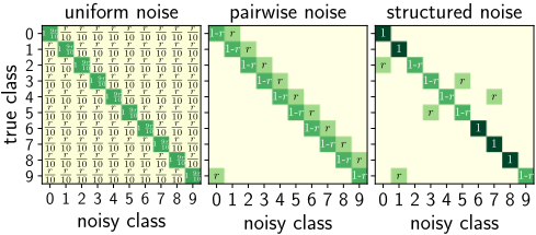
Datasets. The CIFAR-10/100 datasets contain 50K (10K) images for training (test). We retain 5K of the training set for validation following [Tanaka et al., 2018]. For label noise addition, we follow the common criteria in previous works [Patrini et al., 2017; Han et al., 2018b]. Uniform noise is introduced by randomly flipping each label to one of 10/100 classes for CIFAR-10/100 with probability r. For pairwise noise, each class is circularly flipped to the next class with probability r for CIFAR-10/100. We additionally synthesize structured noise for CIFAR-10 following [Patrini et al., 2017], which mimics realistic noise taking place in similar classes: truck → automobile, bird → airplane, deer → horse, cat ↔ dog with transition parameter r. The sketch map for these label noise types for CIFAR-10 is shown in Figure 1. The WebVision [Li et al., 2017] dataset contains 2.4M noisy labeled images crawled from Flickr and Google by using 1,000 concepts in ILSVRC-2012 [Deng et al., 2009] as queries and the overall noise rate is rough 20%. Following [Chen et al., 2019], we use the first 50 classes of Google image subset for training and test on the corresponding 50 classes of WebVision and ILSVRC-2012 validation set.
Baselines. In this paper, we mainly contrast to state-ofthe-art sample selection-based methods: Co-teaching [Han et al., 2018b], Co-teaching+ [Yu et al., 2019], INCV [Chen et al., 2019] and JoCoR [Wei et al., 2020]. We also implement "Cross Entropy" method, which does not use any special treatments for label noise. Additionally, we also compare with LDMI [Xu et al., 2019] on CIFAR-10. Since LDMI can not be used for datasets with a large number of classes, we compare with Truncated Lq [Zhang and Sabuncu, 2018] on CIFAR-100.
5.1 Empirical Findings
We verify our theoretical explanation with the following empirical findings on synthetic CIFAR-10 with different noise types and levels. Due to space limit, detailed experimental settings and more discussions can be found in Appendix B.
Figure 2 implies that when the diagonally-dominant condition is not satisfied, incorrect examples may even have relative smaller loss than correct ones (see Figure 2 (b) r = 0.5 and r = 0.6, (c) r = 0.5 and r = 0.6), which verifies the necessity of this condition for learning from noisy labels with small-loss criterion. Figure 3 shows that the losses for different classes are not comparable, especially for more realistic structured label noise, which justifies the necessity of ranking the losses of examples class by class when selecting smallloss examples. Figure 4 shows that there exist large fluctuations for single epoch's loss, while for the mean loss, the value of the correct example (˜ y = y) is steadily smaller than that of the incorrect one (˜ y ̸= y). It justifies the effectiveness of using the mean loss for small-loss criterion. Theorem 2 implies that the distance between the model g and g∗ is important. In general, when trained with a bigger training set sampled from the noisy data distribution, the model g will be closer to g∗ . Thus we train models using different sizes of the training set to simulate different g with different distances to g∗ , and show the training dynamics and performances in Figure 5. It can be found when g is closer to g∗ , the loss dataset size gap is bigger and the precision of the selected data is higher, which verifies that the small-loss criterion will have better utility when the model g is closer to g∗ . To further verify the effectiveness of the reformalization of small-loss criterion, we compare the precision of the selected data with different methods. In Algorithm 1, we propose to select less data than 1-η for safety, where η is the overall noise rate. But in here for fair comparison, we set the selected proportion as 1 - η for all methods. Since the selected proportions of INCV and Co-teaching+ depend on the algorithms and can not be manually set, we only compare with Co-teaching and JoCoR. As shown in Table 1, by comparing "Only Mean Loss" and "Our Method" with Co-teaching and JoCoR on all noise settings especially for structured noise (CIFAR-10), the effectiveness of "mean loss" and "selecting class by class" are verified respectively.
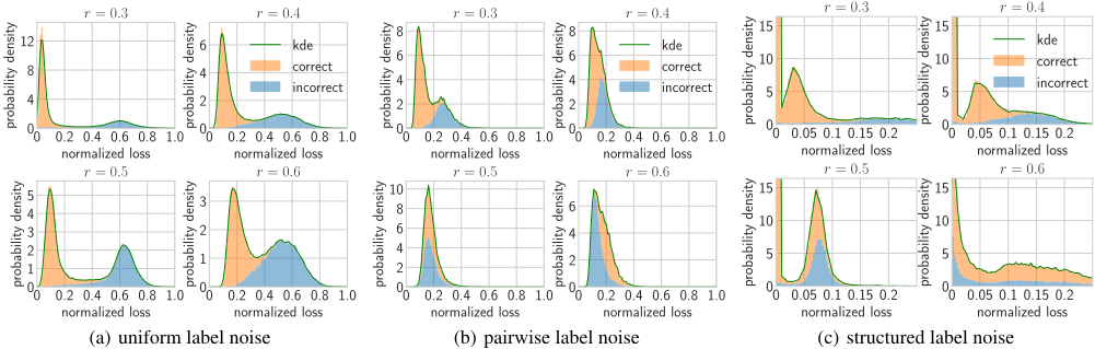
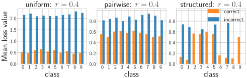
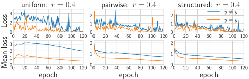
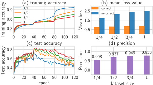
Figure 5: Training accuracy and test accuracy of each epoch in the training process, the mean loss values for correct examples and incorrect ones, and the precision of the selected data (all with the same selection ratio) when using 1 4 , 12 , 34 and 1 of the original noisy training set (uniform noise: r = 0.4) respectively.
5.2 Evaluation on Benchmark Datasets
We evaluate the performance of the proposed method on benchmark datasets. As that in Co-teaching, Co-teaching+
| Method | CIFAR-10 | CIFAR-100 | |||||||||||||||||||
|---|---|---|---|---|---|---|---|---|---|---|---|---|---|---|---|---|---|---|---|---|---|
| uniform noise | pairwise noise | structured noise | uniform noise | pairwise noise | |||||||||||||||||
| noise parameter r (%) | 10 | 30 | 50 | 70 | 90 | 10 | 20 | 30 | 40 | 10 | 20 | 30 | 40 | 20 | 40 | 60 80 | 10 | 20 | 30 | 40 | |
| Co-teaching | 98.58 | 95.32 | 92.25 | 85.32 | 32.68 | 98.01 | 95.61 | 93.42 | 81.36 | 98.19 | 96.55 | 95.04 | 90.58 | 96.30 | 92.34 | 85.37 | 33.38 | 92.38 | 86.73 | 77.30 | 65.21 |
| JoCoR | 98.89 | 96.03 | 93.14 | 86.47 | 20.29 | 98.27 | 96.29 | 93.75 | 82.73 | 98.47 | 96.85 | 95.26 | 91.69 | 96.64 | 92.62 | 86.70 | 40.78 | 94.42 | 88.39 | 79.89 | 67.71 |
| Only Mean Loss | 99.01 | 97.46 | 94.59 | 88.31 | 46.72 | 98.74 | 97.33 | 94.12 | 84.60 | 98.58 | 97.08 | 95.37 | 91.98 | 97.01 | 93.43 | 87.87 | 65.11 | 95.80 | 89.72 | 81.22 | 68.77 |
| Our Method | 99.09 | 97.47 | 94.65 | 88.38 | 46.91 | 98.81 | 97.43 | 94.69 | 84.68 | 99.81 | 99.38 | 97.97 | 94.96 | 97.22 | 93.70 | 88.34 | 66.12 | 95.98 | 90.29 | 82.00 | 69.69 |
| Method | uniform noise | pairwise noise | structured noise | |||||||||||
|---|---|---|---|---|---|---|---|---|---|---|---|---|---|---|
| noise parameter r (%) | 10 | 30 | 50 | 70 | 90 | 10 | 20 | 30 | 40 | 10 | 20 | 30 | 40 | |
| Cross Entropy | best | 91.24 | 88.30 | 84.85 | 78.13 | 44.90 | 91.32 | 90.83 | 88.96 | 83.20 | 91.80 | 90.95 | 88.87 80.26 | 86.57 |
| last | 86.70 | 72.12 | 55.24 | 32.97 | 19.45 | 85.59 | 78.83 | 67.70 | 56.12 | 89.70 | 84.89 | 75.76 | ||
| LDMI | best last | 90.47 | 87.76 | 84.12 | 77.85 | 36.71 | 91.13 | 90.90 | 89.12 | 85.56 | 91.14 | 90.19 | 88.41 | 86.72 86.25 |
| best | 90.07 90.60 | 87.74 89.83 | 84.10 85.14 | 77.73 65.76 | 36.37 11.70 | 91.03 91.59 | 90.45 89.42 | 88.87 87.37 | 85.32 78.18 | 90.28 90.72 | 89.43 89.67 | 88.13 87.12 | 80.59 | |
| Co-teaching | last | 90.36 | 88.98 | 85.09 | 65.65 | 11.69 | 90.71 | 89.02 | 87.24 | 71.76 | 90.35 | 89.63 | 86.73 | 77.81 |
| Co-teaching+ | best | 90.93 | 89.98 | 86.52 | 10.74 | 91.52 | 90.22 | 87.55 | 82.15 | 90.29 | 88.17 | 81.46 | ||
| last best | 90.90 91.82 | 89.36 90.72 | 86.48 86.34 | 77.44 77.38 73.11 | 10.54 38.38 | 91.30 91.42 | 89.37 89.26 | 87.30 87.84 | 81.47 85.73 | 91.28 90.65 91.85 | 90.05 90.58 | 87.44 87.89 | 80.28 86.43 | |
| INCV | last best | 91.79 92.30 | 89.48 89.52 | 86.43 87.27 | 72.78 79.57 | 38.29 26.38 | 91.37 91.87 | 89.19 90.38 | 87.50 88.42 | 85.18 83.48 | 91.62 92.02 | 90.14 90.87 | 87.68 88.78 88.04 | 86.23 83.59 |
| JoCoR | last | 92.28 | 89.48 | 85.86 | 79.62 | 25.18 | 91.82 | 90.32 | 87.44 | 83.42 | 91.99 | 90.23 | 89.97 | 83.40 |
| RSL | best | 93.32 93.23 | 91.34 91.13 | 88.21 87.93 | 82.21 | 39.75 39.54 | 92.71 92.47 | 91.13 90.89 | 90.51 90.31 | 86.73 86.57 | 92.58 92.42 | 91.32 91.24 | 89.83 | 87.91 |
| best | 94.15 | 93.78 | 93.38 | 48.33 | 94.08 | 93.73 | 89.27 | 93.57 | 93.12 | 92.78 | 87.85 91.17 | |||
| RSL WM | last | 93.42 | 93.27 | 82.08 91.51 | 93.40 | 90.63 | ||||||||
| last | 93.59 | 91.31 | 47.43 | 93.21 | 93.19 | 93.10 | 88.85 | 93.33 | 92.83 | 92.34 | ||||
| Method | uniform noise | pairwise noise | |||||||
|---|---|---|---|---|---|---|---|---|---|
| noise parameter r (%) | 20 | 40 | 60 | 80 | 10 | 20 | 30 | 40 | |
| Cross Entropy | best | 62.61 | 53.00 | 42.74 | 29.08 | 68.18 | 64.31 | 59.05 | 45.70 |
| last | 57.44 | 41.96 | 26.05 | 12.76 | 67.24 | 61.13 | 54.03 | 44.44 | |
| Truncated Lq | best | 67.41 | 62.77 | 54.60 | 19.47 | 68.93 | 67.36 | 62.21 | 46.89 |
| last | 66.48 | 62.28 | 53.48 | 17.48 | 68.80 | 67.06 | 62.12 | 45.97 | |
| Co-teaching | best | 69.94 | 63.65 | 54.64 | 12.75 | 68.74 | 67.91 | 62.66 | 50.44 |
| last | 69.53 | 63.23 | 53.57 | 11.27 | 68.46 | 66.24 | 61.84 | 48.83 | |
| Co-teaching+ | best | 65.43 | 63.21 | 54.33 | 11.52 | 67.53 | 64.83 | 59.75 | 46.33 |
| last | 64.74 | 62.69 | 52.23 | 10.57 | 67.37 | 64.26 | 58.59 | 45.67 | |
| INCV | best | 62.68 | 59.78 | 41.39 | 23.43 | 63.93 | 56.68 | 50.87 | 38.95 |
| last | 62.65 | 59.69 | 41.24 | 23.32 | 63.87 | 56.48 | 50.81 | 38.84 | |
| JoCoR | best | 71.40 | 66.80 | 58.40 | 23.44 | 72.31 | 67.92 | 63.38 | 54.37 |
| last | 70.62 | 66.10 | 57.65 | 23.36 | 71.81 | 67.32 | 62.79 | 53.74 | |
| best | 72.12 | 67.23 | 59.24 | 38.32 | 72.42 | 68.43 | 62.45 | 53.62 | |
| RSL | last | 71.84 | 67.03 | 58.78 | 38.04 | 72.46 | 68.27 | 62.23 | 53.25 |
| RSL WM | best | 74.88 | 71.51 | 67.25 | 49.58 | 74.48 | 71.18 | 64.67 | 54.34 |
| last | 73.92 | 70.69 | 66.07 | 49.17 | 73.77 | 70.54 | 63.87 | 53.65 | |
and JoCoR, we also assume that the noise rates are known and put sensitivity analysis of our method on noise rates in Appendix C. We use the default parameters β = 0.2, γ = (γ0+γ1)/2 and κ = - log(0.7) in experiments. Due to space limit, we put all the implementation details and sensitivity analysis on β, γ and κ in Appendix C. For CIFAR-10 and CIFAR-100, as shown in Tables 2 and 3, RSL WM achieves the best performance in almost all noise settings. Although we select less data than Co-teaching and JoCoR, learning only with the selected data (RSL) still gets better accuracy than the compared methods in most cases. By exploiting the information of the unselected data with Weighted MixMatch, better performance is achieved, which verifies the effectiveness of this framework. In the pairwise noise (r = 0.4) on CIFAR-100, our method is less competitive due to we select much less data than JoCoR. For WebVision, we select the first 76% (β = 0.2) examples with small mean loss for each class. We also compare with F-correction [Patrini et al., 2017], MentorNet [Jiang et al., 2018], and D2L [Ma et al., 2018] since they have the same experimental setting as ours. As shown in Table 4, our method achieves better performance than the compared methods.
| Method | WebVision Val. | ILSVRC2012 Val. | ||
|---|---|---|---|---|
| top1 | top5 | top1 | top5 | |
| Cross Entropy | 58.24 | 79.26 | 54.83 | 77.70 |
| F-correction | 61.12 | 82.68 | 57.36 | 82.36 |
| Co-teaching | 63.58 | 85.20 | 61.48 | 84.70 |
| MentorNet | 63.00 | 81.40 | 57.80 | 79.92 |
| D2L | 62.68 | 84.00 | 57.80 | 81.36 |
| Co-teaching+ | 63.21 | 84.78 | 61.32 | 83.52 |
| INCV | 65.24 | 85.34 | 61.60 | 84.38 |
| JoCoR | 65.28 | 85.38 | 61.54 | 84.46 |
| RSL | 65.64 | 85.72 | 62.04 | 84.84 |
| RSL WM | 66.56 | 86.54 | 63.40 | 85.43 |
6 Conclusion
In this paper, we establish the connection between noisy data distribution and the small-loss criterion and theoretically explain why the widely-used small-loss criterion works. In the future, we will consider extending the theoretical explanation to the instance-dependent label noise [Xia et al., 2020].
Acknowledgments
This work is supported by the National Key Research and Development Program of China (2017YFB1002201), the National Science Foundation of China (61921006, 61673202), and the Collaborative Innovation Center of Novel Software Technology and Industrialization.
@inproceedings{ijcai2021p340,
  title     = {Towards Understanding Deep Learning from Noisy Labels with Small-Loss Criterion},
  author    = {Gui, Xian-Jin and Wang, Wei and Tian, Zhang-Hao},
  booktitle = {Proceedings of the Thirtieth International Joint Conference on
               Artificial Intelligence, {IJCAI-21}},
  publisher = {International Joint Conferences on Artificial Intelligence Organization},
  editor    = {Zhi-Hua Zhou},
  pages     = {2469--2475},
  year      = {2021},
  month     = {8},
  note      = {Main Track},
  doi       = {10.24963/ijcai.2021/340},
  url       = {https://doi.org/10.24963/ijcai.2021/340},
}
TY - CPAPER TI - Towards Understanding Deep Learning from Noisy Labels with Small-Loss Criterion AU - Gui, Xian-Jin AU - Wang, Wei AU - Tian, Zhang-Hao T2 - Proceedings of the Thirtieth International Joint Conference on Artificial Intelligence, IJCAI-21 PB - International Joint Conferences on Artificial Intelligence Organization PY - 2021 SP - 2469 EP - 2475 DO - 10.24963/ijcai.2021/340 UR - https://doi.org/10.24963/ijcai.2021/340 ER -Copied
Machine-readable versions of this paper, for tools and AI agents:





