
Boosting Variational Inference With Locally Adaptive Step-Sizes
Proceedings of the Thirtieth International Joint Conference on Artificial Intelligence. Main Track. Pages 2337-2343.
https://doi.org/10.24963/ijcai.2021/322
Keywords
- Machine Learning: Probabilistic Machine Learning
- Machine Learning: Bayesian Learning
Abstract
Variational Inference makes a trade-off between the capacity of the variational family and the tractability of finding an approximate posterior distribution. Instead, Boosting Variational Inference allows practitioners to obtain increasingly good posterior approximations by spending more compute. The main obstacle to widespread adoption of Boosting Variational Inference is the amount of resources necessary to improve over a strong Variational Inference baseline. In our work, we trace this limitation back to the global curvature of the KL-divergence. We characterize how the global curvature impacts time and memory consumption, address the problem with the notion of local curvature, and provide a novel approximate backtracking algorithm for estimating local curvature. We give new theoretical convergence rates for our algorithms and provide experimental validation on synthetic and real-world datasets.
- [Blei et al., 2017] David M. Blei, Alp Kucukelbir, and Jon D. McAuliffe. Variational Inference: A Review for Statisticians. Journal of the American Statistical Associa- tion, 2017.
- [Boyd and Vandenberghe, 2004] Stephen P Boyd and Lieven Vandenberghe. Convex optimization. Cambridge Univer- sity Press, 2004.
- [Burda et al., 2015] Yuri Burda, Roger Grosse, and Rus- lan Salakhutdinov. Importance weighted autoencoders. arXiv:1509.00519, 2015.
- [Campbell and Li, 2019] Trevor Campbell and Xinglong Li. Universal Boosting Variational Inference. NeurIPS, 2019.
- [Cranko and Nock, 2019] Zac Cranko and Richard Nock. Boosted Density Estimation Remastered. ICML, 2019.
- [Fortuin et al., 2019] Vincent Fortuin, Matthias Hüser, Francesco Locatello, Heiko Strathmann, and Gunnar Rätsch. SOM-VAE: Interpretable Discrete Representation Learning on Time Series. ICLR, 2019.
- [Goldberger et al., 2000] Ary L. Goldberger, Luis A. N. Amaral, Leon Glass, Jeffrey M. Hausdorff, Plamen Ch. Ivanov, Roger G. Mark, Joseph E. Mietus, George B. Moody, Chung-Kang Peng, and H. Eugene Stanley. Phys- ioBank, PhysioToolkit, and PhysioNet. Circulation, 2000.
- [Guo et al., 2016] Fangjian Guo, Xiangyu Wang, Kai Fan, Tamara Broderick, and David B Dunson. Boosting Varia- tional Inference. arXiv:1611.05559, 2016.
- [Jaakkola and Jordan, 1998] Tommi S. Jaakkola and Michael I. Jordan. Improving the Mean Field Approxi- mation via the Use of Mixture Distributions. Learning in Graphical Models, 1998. DOI
- [Jaggi, 2013] Martin Jaggi. Revisiting Frank-Wolfe: Projection-Free Sparse Convex Optimization. Interna- tional Conference on Machine Learning (ICML), 2013.
- [Jerfel, 2017] Ghassen Jerfel. Boosted Stochastic Backprop- agation for Variational Inference. Masters Thesis, 2017. [Online; accessed 11. Sep. 2019].
- [Jordan et al., 1999] Michael I Jordan, Zoubin Ghahramani, Tommi S Jaakkola, and Lawrence K Saul. An introduc- tion to variational methods for graphical models. Machine learning, 1999.
- [Lin et al., 2019] Wu Lin, Mohammad Emtiyaz Khan, and Mark Schmidt. Fast and Simple Natural-Gradient Varia- tional Inference with Mixture of Exponential-family Ap- proximations. Proceedings of the 36th International Con- ference on Machine Learning (ICML), 2019.
- [Locatello et al., 2017] Francesco Locatello, Rajiv Khanna, Michael Tschannen, and Martin Jaggi. A Unified Op- timization View on Generalized Matching Pursuit and Frank-Wolfe. In Proc. International Conference on Ar- tificial Intelligence and Statistics (AISTATS), 2017.
- [Locatello et al., 2018a] Francesco Locatello, Gideon Dres- dner, Rajiv Khanna, Isabel Valera, and Gunnar Rätsch. Boosting black box variational inference. In Conference on Neural Information Processing Systems (NeurIPS), 2018.
- [Locatello et al., 2018b] Francesco Locatello, Rajiv Khanna, Joydeep Ghosh, and Gunnar Rätsch. Boosting Variational Inference: an Optimization Perspective. Proceedings of the 21st International Conference on Artificial Intelligence and Statistics (AISTATS 2018), 2018.
- [Locatello et al., 2018c] Francesco Locatello, Damien Vin- cent, Ilya Tolstikhin, Gunnar Rätsch, Sylvain Gelly, and Bernhard Schölkopf. Competitive Training of Mixtures of Independent Deep Generative Models. Workshop at the 6th International Conference on Learning Representations (ICLR), 2018.
- [Meir and Rätsch, 2003] Ron Meir and Gunnar Rätsch. An introduction to boosting and leveraging. In Advanced lec- tures on machine learning. Springer, 2003.
- [Miller et al., 2017] Andrew C Miller, Nicholas Foti, and Ryan P Adams. Variational Boosting: Iteratively Refining Posterior Approximations. Proceedings of the 34th Inter- national Conference on Machine Learning (ICML), 2017.
- [Nesterov, 2018] Yurii Nesterov. Lectures on convex opti- mization. Springer, 2018. DOI
- [Paquette and Scheinberg, 2018] Courtney Paquette and Katya Scheinberg. A Stochastic Line Search Method with Convergence Rate Analysis. arXiv:1807.07994, 2018.
- [Pedregosa et al., 2020] Fabian Pedregosa, Armin Askari, Geoffrey Negiar, and Martin Jaggi. Linearly Convergent Frank-Wolfe with Backtracking Line-Search. Proceedings of the 22nd International Conference on Artificial Intelli- gence and Statistics, 2020.
- [Rezende and Mohamed, 2015] Danilo Jimenez Rezende and Shakir Mohamed. Variational Inference with Nor- malizing Flows. In Proceedings of the 32nd International Conference on Machine Learning (ICML), 2015.
- [Saeedi et al., 2017] Ardavan Saeedi, Tejas D. Kulkarni, Vikash K. Mansinghka, and Samuel J. Gershman. Vari- ational Particle Approximations. Journal of Machine Learning Research, 2017.
- [Salimans et al., 2015] Tim Salimans, Diederik P. Kingma, and Max Welling. Markov Chain Monte Carlo and Vari- ational Inference: Bridging the Gap. Proceedings of the 32nd International Conference on Machine Learning (ICML), 2015.
- [Saxena et al., 2017] Siddhartha Saxena, Shibhansh Dohare, and Jaivardhan Kapoor. Variational Inference via Trans- formations on Distributions. CoRR, 2017.
- [Tran et al., 2016] Dustin Tran, Alp Kucukelbir, Adji B. Di- eng, Maja Rudolph, Dawen Liang, and David M. Blei. Ed- ward: A library for probabilistic modeling, inference, and criticism. arXiv:1610.09787, 2016.
References were extracted automatically from the PDF and may contain errors.
Full text extracted automatically from the PDF; figures, tables and equations may differ. The PDF is the version of record.
1 Introduction
The central problem of Bayesian inference is to estimate the posterior distribution p(z|X) of hidden variables z, given observations X, a likelihood model p(X|z), and a prior distribution p(z). The Variational Inference (VI) approach [Jordan et al., 1999; Blei et al., 2017] consists in finding the best approximation in Kullback-Leibler (KL)-divergence to the posterior from within a family of tractable densities Q. This is posed as the following optimization problem:
We occasionally abuse the notation for DKL: When the target distribution is omitted, as above, it is understood that the target is the true posterior distribution p(z|X).
There is a trade-off between the quality of the approximation and the difficulty of the optimization problem. While a richer family may yield a better approximation of the posterior, finding such a solution requires solving a more complex optimization problem. A growing body of recent work addresses this trade-off by specifying variational families that are richer but still tractable [Rezende and Mohamed, 2015; Saeedi et al., 2017; Salimans et al., 2015; Saxena et al., 2017; Cranko and Nock, 2019]. However, once the VI solver has converged, one cannot spend more compute to improve the approximation. If the approximation is too poor to be useful, it must be abandoned and the inference procedure restarted with a richer variational family.
A full version of this paper including the appendix is available
at https://arxiv.org/abs/2105.09240.
The recent line of work in Boosting VI takes a different approach. Instead of specifying a richer variational family, Boosting VI greedily constructs one using mixtures of densities from a simpler base family [Guo et al., 2016; Miller et al., 2017; Locatello et al., 2018b; Locatello et al., 2018a; Cranko and Nock, 2019]. The key idea is that one can iteratively build a better approximation to the target posterior by fitting the residual parts which are not yet well-approximated.
Despite advances in making boosting agnostic to the choice of the variational family [Locatello et al., 2018a], this line of work has fallen short of its potential. The reason for this is that Boosting VI does not reliably improve the variational approximation in a reasonable number of iterations [Guo et al., 2016; Locatello et al., 2018b; Locatello et al., 2018a].
In this work, we present a new technique for determining the mixture weights of Boosting VI algorithms which improves the variational approximation in a realistic number of iterations. As we shall see, the previous convergence rates depend on two terms: a term depending on the global curvature of the KL and the initial error. Practitioners often focus on decreasing the latter term, but the first one can be arbitrarily large without imposing extra assumptions.
We are able to improve the dependency on the curvature in the convergence rate by tuning the mixture weights according to a quadratic function satisfying a sufficient decrease condition, i.e. is sufficiently tight on the KL divergence objective [Pedregosa et al., 2020].
In the black-box VI setting, checking for exact upper bounds is not feasible due to sampling errors. Therefore, we consider the case where the estimate of the bound is inexact. Using this approximate local upper-bound, we develop a fast and memory efficient away-step black-box Boosting VI algorithm.
Our main contributions can be summarized as follows:
- We introduce an approximate sufficient decrease condition
and prove that the resulting backtracking algorithm converges with a rate of O(1/t) with an improved dependency on the curvature constant.
- We develop an away-step Boosting VI algorithm that relies on our approximate backtracking algorithm. This enables Boosting VI methods to selectively downweight previously seen components to obtain sparser solutions, thus reducing overall memory costs.
- We present empirical evidence demonstrating that our method is both faster and more robust than existing methods. The adaptive methods also yield more parsimonious variational approximations than previous techniques.
2 RelatedWork
We refer to [Blei et al., 2017] for a review of Variational Inference (VI). Our focus is to use boosting to increase the complexity of a density, similar to the goal of Normalizing Flows [Rezende and Mohamed, 2015], MCMC-VI hybrid methods [Saeedi et al., 2017; Salimans et al., 2015], distribution transformations [Saxena et al., 2017], and boosted density estimation [Cranko and Nock, 2019; Locatello et al., 2018c]. Our approach is in line with several previous ones using mixtures of distributions to improve the expressiveness of the variational approximation [Jaakkola and Jordan, 1998; Jerfel, 2017] but goes further to draw connections to the optimization literature. While our method does not leverage classical weak learners as in [Cranko and Nock, 2019], it does return a solution which is sampleable and is therefore more amenable to downstream Bayesian analysis.
While boosting has been well studied in other settings [Meir and R¨atsch, 2003], it has only recently been applied to the problem of VI. Related works of [Guo et al., 2016; Miller et al., 2017] developed the algorithmic framework and conjectured a convergence rate of O(1/t). Later, [Locatello et al., 2018b] identified sufficient conditions for convergence and provided explicit constants to the O(1/t) rate. They based their analysis on the smoothness of the KL-divergence when using carefully constructed variational base families which are restrictive in practice.
In [Locatello et al., 2018a], these assumptions were reduced to a simple entropy regularizer which allows for a black-box implementation of the boosting subroutine. The promise of their work is to make Boosting VI useful in practice while retaining an O(1/t) convergence rate.
Recent work by [Campbell and Li, 2019] and [Lin et al., 2019] also explore the relationship between Boosting VI and curvature. In this paper, we present our unique view on curvature which does not require sacrificing the KL-divergence for a smooth objective as in [Campbell and Li, 2019] or fixing the number of components in the mixture [Lin et al., 2019]. Finally, note that [Locatello et al., 2018b] also suggests performing line-search on a quadratic approximation of the KLdivergence. Crucially, they suggest using a global approximation which renders their step-size arbitrarily small. See Table 1 for comparison to prior work.
Backtracking line-search and related variants are wellunderstood for deterministic objectives with projectionable constraints [Boyd and Vandenberghe, 2004]. However, backtracking techniques have only recently been applied to FrankWolfe by [Pedregosa et al., 2020]. Our work lies at the intersection of these developments in VI and backtracking linesearch.
3 Boosting Variational Inference
Boosting Variational Inference (VI) aims to solve an expanded version of the problem defined in Equation (1) by optimizing over the convex hull of Q defined as,
Boosting VI algorithms take a greedy, two-step approach to solving this problem. At each iteration, first, the posterior residual pX/qt is approximated with an element of Q and added to the list of components. Then, the weights of the mixture are updated. Previous research on Boosting VI has focused on the first step - selecting the best fitting density of the residual -whereas our work takes into consideration the second step - adjusting the weights. As we shall see, step-size choice has a significant impact on both the constant in the convergence rate as well as the observed speed in practice.
Selecting the next component. Greedily approximating the residual pX/qt is equivalent to solving a linear minimization problem as first realized by [Guo et al., 2016] and later formalized by [Locatello et al., 2018b]. Our contribution (Sec. 4) can be combined with any of these approaches.
Without imposing additional constraints on the boosted Variational Inference problem, the greedy subproblem has degenerate solutions, i.e. Dirac delta located at the maximum of the residual [Locatello et al., 2018b; Locatello et al., 2018a; Guo et al., 2016; Miller et al., 2017]. This is the central challenge addressed by existing work on Boosting Variational Inference. The approach taken in [Locatello et al., 2018a] is to use a generic entropy regularizer as the additional constraint. This conveniently reframes the subproblem as another KLminimization problem which can then be fed into existing black-box VI solvers.
In their work, the greedy step can be formulated as a constrained linear minimization problem over the variational family,
where H is the differential entropy functional. This results in a modified overall Variational Inference objective over the entropy constrained mixtures, rather than all of conv(Q):
where Q def = {s ∈ Q | H(s) ≥ -M}.
By reformulating the differential entropy constraint in Equation (2) using a Lagrange multiplier and then setting the multiplier to one, one arrives at a convenient form for the greedy subproblem (Alg. 1 line 3):

Intuitively, this objective encourages the next component to be close to the target posterior lnpX while simultaneously being different from current iterate lnqt and also being nondegenerate via the negative entropy term ln s.
Predefined step-size. To update the mixture, [Locatello et al., 2018a] take a convex combination between the current approximation and the next component (Alg. 1 line 7) with a predefined step-size of γt = 2 t+2 :
where vt is set to qt.
4 Local Boosting Variational Inference
We now describe our main algorithmic contribution.
Notation. We view expectations as a special case of functional inner-products. Given two functionals, a, b : z ↦→ R, their inner-product is 〈a, b〉 def = ∫ a(z)b(z)dz. Practically, we only encounter these integrals when one of the arguments is a density that can be sampled from thus allowing us to use Monte-Carlo: 〈a, b〉 ≈̂ 〈a, b〉 def = 1n ∑ki=1 b(ζi) where ζi ∼ a.
Assumption. We assume that for all ε > 0 there exists an n ∈ N number of Monte-Carlo samples such that for all s ∈ Q and q ∈ conv(Q), the Monte-Carlo approximation 〈s,∇DKL(q)〉∧is ε-close to the true value:
This assumption states that we can approximate the value of the objective in Equation (2) up to a predefined tolerance.
Now, suppose we are at iteration t of the boosting algorithm (Alg. 1). qt is the current variational approximation containing at most t components. The next component st is provided by line 3. vt is then returned from the corrective components procedure (described in Sec. 4.1 and App. A). Let dt = st - vt be the update direction.
Our goal is to solve the following one dimensional prob-
lem, Then we can set qt+1 = qt + γtdt as described in line 7 of Algorithm 1. Solving this problem - often termed "line-search" - may be hard when no closed-form solution is available e.g. in the case of black-box VI [Locatello et al., 2017; Locatello et al., 2018b; Locatello et al., 2018a; Pedregosa et al., 2020]. In practice, general approaches such as gradient descent struggle to handle the changing curvature of the KL-divergence throughout conv(Q) (c.f. Sec. 6).
Instead, [Pedregosa et al., 2020] uses so-called DeminovRubinov line-search. Rather than solving the line-search problem directly, their technique defines a surrogate objective:
Importantly, there exists Ct > 0 such that for all γ ∈ [0, 1], Qt(γ,Ct) is a valid upper bound on the line-search problem (Eq. (7)). In this case, we say that Ct satisfies the sufficient decrease condition:
Essentially, we are bounding the first-order Taylor expansion of the KL-divergence at qt + γdt (as in Eq. (7)).
Unlike the finite dimensional setting described in [Pedregosa et al., 2020], in black-box VI we are unable to validate the sufficient decrease condition directly because we can only approximate Qt within a precision of εt,
where ̂Qt is theMonte-Carlo approximation toQt. This leads us to define an approximate sufficient decrease condition (c.f. Appendix B.3):
where εt = O(1/t2 ). If we assume that the number of samples is large enough, then we can guarantee that
Intuitively, we are adding an offset of εt to compensate for errors in the Monte-Carlo approximation of Qt. As we will
Algorithm 1 Template for Boosting VI algorithms
1: Input: q0 ∈ Q, C-1 > 0 2: for t = 0, 1 . . . do 3: st = argmins∈QDKL(s‖ pX qt ) {next component} 4: vt, γmax t = CORRECT COMPONENTS(st, qt) 5: γt,Ct = FIND STEP SIZE(qt, st - vt,Ct-1, γmax t ) 6: Update: qt+1 = qt +γt(st - vt) 7: end forAlgorithm 2 Find step-size with approximate backtracking
- 1: function FIND STEP SIZE(qt, dt,C, γmax t ) 2: Choose: τ > 1, η ≤ 1, ε0 > 0, IMAX ∈ Z+ 3: Let: gt = -〈∇DKL(qt), dt〉 4: Set: C ←C/η, γ =min{gt/C, 1}, i = 0 5: whilê DKL(qt + γdt) > ̂Q′t (γ, C) do 6: if i > IMAX then 7: return 2 t+2 , C {predefined step-size} 8: end if 9: C ← τC 10: γ = min{gt/C, γmax t } 11: i ← i + 1 12: end while 13: return γ,C {adaptive step-size} 14: end function
see in Section 5, to obtain an overall convergence rate we require that εt decreases at each iteration. Equivalently, this requires increasing the number of samples at each step of the algorithm.
Suppose that, for some Ct, ̂Q′t satisfies the approximate sufficient decrease condition. Then, ̂Q′t (γ,Ct) can easily be minimized with respect to γt by setting the derivative with respect to γ equal to zero and solving:
where γmax t ∈ (0, 1] depends on the corrective algorithm variant (c.f. Sec. 4.1). Equation (13) shows that Ct and γt are inversely proportional. Intuitively, the new component should be aggressively favored when it is highly correlated with the gradient of the KL-divergence since this gradient is the optimal decrease direction. We want to take advantage of these low curvature opportunities to take more aggressive steps towards improving the posterior approximation.
Therefore, our goal is to find a Ct which satisfies the approximate sufficient decrease conditions of Equation 9 while also being as small as possible. This is achieved using approximate backtracking on C (Alg. 2).
The cost of this procedure is the cost of estimating the sufficient decrease condition for each proposal of Ct. The MonteCarlo estimates used to compute ̂Q′t can be reused but the approximation to DKL(qt + γdt) must be re-estimated.
Observe that in order to guarantee convergence, there must exist a global bound on Ct. This quantity is known as the global curvature and is defined directly as the supremum over all possible Ct's [Jaggi, 2013]:
Section 5.1 provides theoretical results clarifying the relationship between Ct and CQ.
We make a slight modification to the algorithm to circumvent this problem, summarized in lines (6-8) of Algorithm 2. When the adaptive loop fails to find an approximation within IMAX number of steps, it exits and simply performs a predefined step-size update. We find that this trick allows us to quickly escape from curved regions of the space. After just one or two predefined update steps, we can efficiently estimate the curvature and apply the approximate backtracking procedure. See Appendix C for results on early termination.
4.1 Correcting the Current Mixture
Not only does our work analyze and solve the problem of varying curvature in Boosting VI, it also enables the use of more sophisticated, corrective variants of the boosting algorithm. Corrective variants aim to address the problem of downweighting or removing suboptimally chosen components. This is important in the approximate regime of VI where most quantities are estimated using Monte-Carlo. However, it is impossible to apply these corrective methods to boosting without a step-size estimation method such as we describe in Section 4.
In the optimization literature, there are two corrective methods (c.f. App. A). Either one of these variants can be substituted for the CORRECT COMPONENTS procedure. Both corrective methods begin by searching for the worst previous component, v in the sense of most closely aligning with the positive gradient of the current approximation:
where St = {s1, s2, . . . , sk} is the current set of components. ¯ v is found by estimating each element of St using MonteCarlo samples and selecting the argmax.
Implementation. Using the work of [Locatello et al., 2018a], we perform the greedy step using existing Variational Inference techniques. For example, if Q is a reparameterizable family of densities, then the reparameterization trick can be used in conjugation with gradient descent methods on the parameters of s ∈ Q. All the quantities necessary to compute ̂Q′t , γt, and ¯ v, are estimated using Monte-Carlo.
5 Convergence Analysis
The following theorem shows a convergence rate for our algorithm. It extends the work of [Pedregosa et al., 2020] to the case of Variational Inference
Theorem 1. Let qt be the t-th iterate generated by Algorithm 1. Let εt = ε0 t2 bound the Monte-Carlo approximation error, described in Equation (6), with some initial approximation error ε0 > 0. Let Ct def = 1t ∑t-1 i=0 Ct be the average of
the curvature constant estimates. Then we have:
| Train LL | Test AUROC | Time (in s) | |
|---|---|---|---|
| AdaAFW | -0.669 ± 5.390e-04 | 0.787 ± 4.599e-03 | 48.240 ± 2.384e+01 |
| AdaPFW | -0.672 ± 6.340e-04 | 0.791 ± 2.398e-03 | 107.247 ± 1.675e+02 |
| AdaFW | -0.671 ± 9.700e-04 | 0.789 ± 7.985e-03 | 40.870 ± 1.647e+01 |
| Predefined∗ | -0.676 ± 7.435e-04 | 0.788 ± 7.401e-03 | 7.296 ± 1.777e+00 |
| Line-search | -0.669 ± 1.011e-03 | 0.791 ± 7.514e-03 | 265.608 ± 1.655e+02 |
| Train LL | Test AUROC | Time (in s) | |
|---|---|---|---|
| AdaAFW | -0.169 ± 1.111e-03 | 0.859 ± 2.565e-03 | 74.634 ± 3.369e+01 |
| AdaPFW | -0.172 ± 1.361e-03 | 0.857 ± 1.011e-03 | 149.721 ± 1.088e+02 |
| AdaFW | -0.170 ± 1.774e-03 | 0.859 ± 3.672e-03 | 54.334 ± 2.632e+01 |
| Predefined∗ | -0.181 ± 2.983e-03 | 0.853 ± 3.693e-03 | 21.369 ± 9.631e+00 |
| Line-search | -0.181 ± 2.651e-03 | 0.854 ± 3.473e-03 | 145.725 ± 1.347e+02 |
where E0 def = DKL(q0) -ψ(∇DKL(q0)) is the initialization error (ψ denotes the dual objective) and δ > 0 bounds the error of estimating the greedy subproblem defined in Equation (4). See Appendix B for the proof.
It is clear that the Monte-Carlo estimates must be increasingly accurate at each iteration to guarantee convergence. This can be achieved by increasing the number of samples.
The average Ct will be kept much smaller than the global curvature CQ. Previous results give rates in terms of global curvature [Locatello et al., 2018a; Locatello et al., 2018b; Guo et al., 2016; Campbell and Li, 2019]. Without making additional assumptions, the global curvature is in principle unbounded. This explains why the number of iterations t must be large before observing the decrease in the error expected from prior work.
5.1 Discussion
The authors of [Locatello et al., 2018a; Locatello et al., 2018b] also provide a convergence rate for their algorithm. However, in practice this rate is never achieved. This is due to a dependence on the global curvature (Eq. (14)) of the KLdivergence which can be huge in certain areas of conv(Q). Since the inner loop of the algorithm is essentially a full run of Variational Inference, it is impossible to run it enough times to beat the global curvature and decrease the initial error as O(1/t).
We reduce the rate by focusing on the curvature constant which, as shown by Equation (13), is directly related to the estimation of the mixture weights. In practice, our approximate backtracking approach on the local curvature is a viable middle ground between exact line-search, which is expensive for the KL divergence, and predefined step-size which requires an infeasibly large number of iterations.
Recognize that the backtracking approach of [Pedregosa et al., 2020] cannot be applied directly to the VI setting because Qt cannot be computed exactly. Overestimation of Qt due to approximation errors results in slower convergence. However, if Ct is underestimated, then the step-size will be overestimated which breaks the convergence proof of [Pedregosa et al., 2020]. By introducing the parameter εt, we can provide some control over this underestimation problem as well as fully characterize the theoretical consequences.
Limitations. Determining the number of samples needed to satisfy the assumption of Section 4, namely, the number of samples needed to guarantee the convergence rate provided in Theorem 1, is a long-standing open problem. There is work on this subject ranging from pure optimization [Paquette and Scheinberg, 2018] to Importance Weighted Autoencoders [Burda et al., 2015]. In this paper, our goal is to characterize the problem theoretically in terms of convergence rates. We believe that this clarifies the ongoing gap between theory and practice. Despite this gap, we found empirically that 100 Monte-Carlo samples was sufficient.
6 Empirical Validation
6.1 Instability of Line-Search
We tested the behavior of gradient-based line-search methods in a well-understood synthetic setup in which the target posterior is a mixture of two Gaussians. We set the first variational component to be the first component of the target density assuming a perfect first iteration. We then compare the performance of step t = 1 of the algorithm, with that of linesearch and our adaptive method at step t = 2, over multiple runs. To measure overall performance, we use (approximate) KL-divergence to the true posterior.
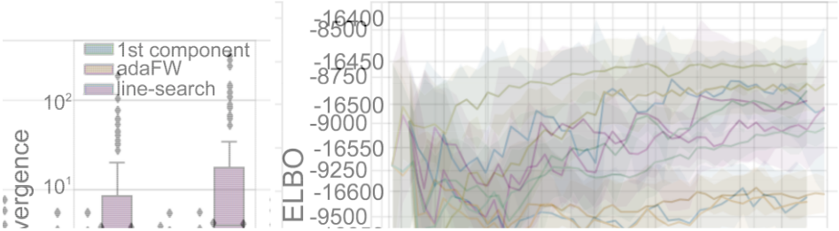
Line-search becomes unstable as the dimensionality increases. This is because line-search oscillates between the two extreme values of zero and one, regardless of the quality of the next component. The quality of the next random component decreases with the dimensionality due to the curse of dimensionality. Even in medium dimensional cases, linesearch is unable to distinguish between these cases. Results are summarized in Figure 1 (left).
Source code to reproduce our experiments is available here: https://github.com/ratschlab/adaptive-stepsize-boosting-bbvi
6.2 Bayesian Logistic Regression
We consider two real-world binary-classification tasks: predicting the reactivity of a chemical and predicting mortality in the intensive care unit (ICU). For both tasks we use Bayesian logistic regression. Bayesian logistic regression is a conditional prediction model with prior p(w) = N(0, 1) and conditional likelihood p(y|X) = Bernoulli(p = sigmoid(X⊤w)). This model is commonly used as an example of a simple model which does not have a closed-form posterior [Blei et al., 2017]. We set the base family to be the Laplace distributions following [Locatello et al., 2018a].
Chemical reactivity. For this task we used the CHEMREACT 1 dataset which contains 26,733 chemicals, each with 100 features. We ran our algorithm multiple times for 50 iterations. We selected the iterate with the best median train log-likelihood over 10 replicates in the first 50 boosting iterations (Table 2).
Mortality prediction. For this task we used the EICU COLLABORATIVE RESEARCH database [Goldberger et al., 2000]. Following [Fortuin et al., 2019], we selected a subset of the data with 71,366 patient stays and 70 relevant features ranging from age and gender to lab test results. We ran boosting for 40 iterations and, for each algorithm, chose the iteration which gave best median train log-likelihood over 10 replicates (Tab. 3).
1 http://komarix.org/ac/ds/
In both datasets, we observe that adaptive variants achieve a better ELBO and are more stable than line-search (Fig. 1 (center and right)). This results in better AUROC and train log-likelihood (Tab. 2, 3).
Naturally, predefined step-size is the fastest since it simply sets the step-size to 2/(t + 2). But, this results in suboptimal performance and unnecessarily large variational approximations. Our approach results in at least a 2x speed-up over line-search as well as better performance.
Adaptive variants are also faster than line-search (Tables 2 and 3). Step-size adaptivity is only 2-5 times slower than predefined step-size as opposed to line-search which is 7-39 times slower. Overall, we observe that step-size adaptivity is faster, more stable, and yields more accurate models than line-search.
6.3 Memory Efficiency
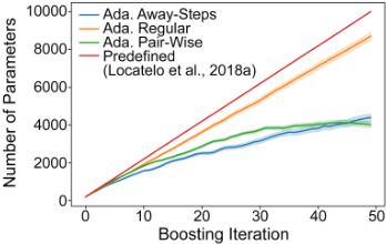
Our corrective methods discussed in Section 4.1 not only yield superior solutions in terms of accuracy, but also yield more parsimonious models by removing previously selected components. Figure 2 demonstrates this behavior on the CHEMREACT dataset. Appendix C has similar results on the EICU dataset.
7 Conclusion
In this paper, we traced the limitations of state-of-the-art boosting variational inference methods back to the global curvature of the KL-divergence. We characterized how the global curvature directly impacts both time and memory consumption in practice, addressed this problem using the notion of local curvature, and provided a novel approximate backtracking algorithm for estimating the local curvature efficiently. Our convergence rates not only provide theoretical guarantees, they also clearly highlight the trade-offs inherent to boosting variational inference. Empirically, our method enjoys improved performance over line-search while requiring significantly less memory consumption than a predefined step-size.
Applying this work to more complex inference problems such as Latent Dirichlet Analysis (LDA) is a promising direction for future work.
@inproceedings{ijcai2021p322,
  title     = {Boosting Variational Inference With Locally Adaptive Step-Sizes},
  author    = {Dresdner, Gideon and Shekhar, Saurav and Pedregosa, Fabian and Locatello, Francesco and Rätsch, Gunnar},
  booktitle = {Proceedings of the Thirtieth International Joint Conference on
               Artificial Intelligence, {IJCAI-21}},
  publisher = {International Joint Conferences on Artificial Intelligence Organization},
  editor    = {Zhi-Hua Zhou},
  pages     = {2337--2343},
  year      = {2021},
  month     = {8},
  note      = {Main Track},
  doi       = {10.24963/ijcai.2021/322},
  url       = {https://doi.org/10.24963/ijcai.2021/322},
}
TY - CPAPER TI - Boosting Variational Inference With Locally Adaptive Step-Sizes AU - Dresdner, Gideon AU - Shekhar, Saurav AU - Pedregosa, Fabian AU - Locatello, Francesco AU - Rätsch, Gunnar T2 - Proceedings of the Thirtieth International Joint Conference on Artificial Intelligence, IJCAI-21 PB - International Joint Conferences on Artificial Intelligence Organization PY - 2021 SP - 2337 EP - 2343 DO - 10.24963/ijcai.2021/322 UR - https://doi.org/10.24963/ijcai.2021/322 ER -Copied
Machine-readable versions of this paper, for tools and AI agents:





