
Likelihood-free Out-of-Distribution Detection with Invertible Generative Models
Proceedings of the Thirtieth International Joint Conference on Artificial Intelligence. Main Track. Pages 2119-2125.
https://doi.org/10.24963/ijcai.2021/292
Keywords
- Uncertainty in AI: Uncertainty Representations
- Data Mining: Anomaly/Outlier Detection
- Machine Learning: Deep Learning
Abstract
Likelihood of generative models has been used traditionally as a score to detect atypical (Out-of-Distribution, OOD) inputs. However, several recent studies have found this approach to be highly unreliable, even with invertible generative models, where computing the likelihood is feasible. In this paper, we present a different framework for generative model--based OOD detection that employs the model in constructing a new representation space, instead of using it directly in computing typicality scores, where it is emphasized that the score function should be interpretable as the similarity between the input and training data in the new space. In practice, with a focus on invertible models, we propose to extract low-dimensional features (statistics) based on the model encoder and complexity of input images, and then use a One-Class SVM to score the data. Contrary to recently proposed OOD detection methods for generative models, our method does not require computing likelihood values. Consequently, it is much faster when using invertible models with iteratively approximated likelihood (e.g. iResNet), while it still has a performance competitive with other related methods.
- [Behrmann et al., 2019] J. Behrmann, W. Grathwohl, R. T. Q. Chen, D. Duvenaud, and J.-H. Jacobsen. Invert- ible residual networks. In International Conference on Machine Learning, pages 573-582. PMLR, 2019.
- [Bishop, 1994] C. M. Bishop. Novelty detection and neural network validation. IEE Proceedings-Vision, Image and Signal processing, 141(4):217-222, 1994.
- [Chen et al., 2019] R. T. Q. Chen, J. Behrmann, D. K. Du- venaud, and J.-H. Jacobsen. Residual flows for invertible generative modeling. In Advances in Neural Information Processing Systems, pages 9916-9926, 2019.
- [Choi et al., 2018] H. Choi, E. Jang, and A. A. Alemi. Waic, but why? generative ensembles for robust anomaly detec- tion. arXiv preprint arXiv:1810.01392, 2018.
- [Dinh et al., 2017] L. Dinh, J. Sohl-Dickstein, and S. Ben- gio. Density estimation using real nvp. In International Conference on Learning Representations, 2017.
- [Erfani et al., 2016] S. M. Erfani, S. Rajasegarar, S. Karunasekera, and C. Leckie. High-dimensional and large-scale anomaly detection using a linear one- class SVM with deep learning. Pattern Recognition, 58:121-134, 2016.
- [Goodfellow et al., 2014] I.
- Goodfellow, J. Pouget-Abadie, M. Mirza, B. Xu, D. Warde-Farley, S. Ozair, A. Courville, and Y. Bengio. Generative adversarial nets. Advances in neural information processing systems, 27:2672-2680, 2014.
- [Kingma and Dhariwal, 2018] D. P. Kingma and P. Dhari- wal. Glow: Generative flow with invertible 1×1 convo- lutions. Advances in Neural Information Processing Sys- tems, (2):10215-10224, 2018.
- [Lakshminarayanan et al., 2017] B. Lakshminarayanan, A. Pritzel, and C. Blundell. Simple and scalable predictive uncertainty estimation using deep ensembles. In Advances in Neural Information Processing Systems, 2017.
- [Lan and Dinh, 2020] C. L. Lan and L. Dinh. Perfect den- sity models cannot guarantee anomaly detection. arXiv preprint arXiv:2012.03808, 2020.
- [Lee et al., 2018] K. Lee, K. Lee, H. Lee, and J. Shin. A simple unified framework for detecting out-of-distribution samples and adversarial attacks. Advances in Neural In- formation Processing Systems, (LID):7167-7177, 2018.
- [Morningstar et al., 2021] W. Morningstar, C. Ham, A. Gal- lagher, B. Lakshminarayanan, A. Alemi, and J. Dillon. Density of states estimation for out of distribution detec- tion. In International Conference on Artificial Intelligence and Statistics, pages 3232-3240. PMLR, 2021.
- [Nalisnick et al., 2019a] E. Nalisnick, A. Matsukawa, Y. W. Teh, D. Gorur, and B. Lakshminarayanan. Do deep gener- ative models know what they don't know? In International Conference on Learning Representations, 2019.
- [Nalisnick et al., 2019b] E. Nalisnick, A. Matsukawa, Y. W. Teh, and B. Lakshminarayanan. Detecting Out-of- Distribution Inputs to Deep Generative Models Using Typ- icality. arXiv preprint arXiv:1906.02994, 2019.
- [Pidhorskyi et al., 2018] S. Pidhorskyi, R. Almohsen, D. A. Adjeroh, and G. Doretto. Generative probabilistic nov- elty detection with adversarial autoencoders. Advances in Neural Information Processing Systems, (NeurIPS):6822- 6833, 2018.
- [Ren et al., 2019] J. Ren, P. J. Liu, E. Fertig, J. Snoek, R. Poplin, M. Depristo, J. Dillon, and B. Lakshmi- narayanan. Likelihood ratios for out-of-distribution detec- tion. In Advances in Neural Information Processing Sys- tems, pages 14707-14718, 2019.
- [Ritter et al., 2018] H. Ritter, A. Botev, and D. Barber. A scalable laplace approximation for neural networks. In 6th International Conference on Learning Representations, ICLR 2018-Conference Track Proceedings, volume 6. In- ternational Conference on Representation Learning, 2018.
- [Ruff et al., 2020] L. Ruff, J. R. Kauffmann, R. A. Van- dermeulen, G. Montavon, W. Samek, M. Kloft, T. G. Dietterich, and K.-R. Müller. A unifying review of deep and shallow anomaly detection. arXiv preprint arXiv:2009.11732, 2020.
- [Sastry and Oore, 2020] C. S. Sastry and S. Oore. Detecting out-of-distribution examples with gram matrices. In Pro- ceedings of the 37th International Conference on Machine Learning, volume 119 of Proceedings of Machine Learn- ing Research, pages 8491-8501. PMLR, 13-18 Jul 2020.
- [Schölkopf et al., 2001] B. Schölkopf, J. C. Platt, J. Shawe- Taylor, A. J. Smola, and R. C. Williamson. Estimating the support of a high-dimensional distribution. Neural Com- putation, 13(7):1443-1471, 2001.
- [Serrà et al., 2020] J. Serrà, D. Álvarez, V. Gómez, O. Sli- zovskaia, J. F. Núñez, and J. Luque. Input complexity and out-of-distribution detection with likelihood-based gener- ative models. In International Conference on Learning Representations, 2020.
- [Steinwart et al., 2005] I. Steinwart, D. Hush, and C. Scovel. A classification framework for anomaly detection. Journal of Machine Learning Research, 6(Feb):211-232, 2005.
- [Winkens et al., 2020] J. Winkens, R. Bunel, A. G. Roy, R. Stanforth, V. Natarajan, J. R. Ledsam, P. MacWilliams, P. Kohli, A. Karthikesalingam, S. Kohl, and Others. Con- trastive training for improved out-of-distribution detection. arXiv preprint arXiv:2007.05566, 2020.
- [Zhai et al., 2016] S. Zhai, Y. Cheng, W. Lu, and Z. Zhang. Deep Structured Energy Based Models for Anomaly De- tection. 33rd International Conference on Machine Learn- ing, ICML, 3:1742-1751, 2016.
- [Zhang et al., 2020] Y. Zhang, W. Liu, Z. Chen, J. Wang, Z. Liu, K. Li, H. Wei, and Z. Chen. Out-of-Distribution Detection with Distance Guarantee in Deep Generative Models. arXiv preprint arXiv:2002.03328, 2020.
References were extracted automatically from the PDF and may contain errors.
Full text extracted automatically from the PDF; figures, tables and equations may differ. The PDF is the version of record.
1 Introduction
Even the machine learning models which have an excellent performance under the assumption 'test data comes from the same distribution as training data' may fail catastrophically (e.g. make a high-confidence false prediction) on an input that is completely different from their training data, such as a noisy observation or rare event of the real environment. This is where Out-of-Distribution (OOD) detection can help and prevent consequent risky decisions. OOD detection is the task of detecting data samples that are dissimilar from the samples in a given (regular) training set of data. Such irregular samples are also called anomalies, novelties, and outliers in the literature, sometimes with slight distinctions, but the term OOD is used in this paper to refer to any type of atypical input presented at 'test time'.
OOD detection can aim at finding either point anomalies or group anomalies [Ruff et al., 2020]. In the former, the input is assumed to be a single data vector, whereas in the latter irregularities are detected by looking at a set of observations. We only address point anomalies in this work, which seems to be a more practical and challenging problem. Moreover, we assume that the problem is completely unsupervised, which means we do not have any examples of OOD data or any other type of class labels at training time. Generative models are a well-known tool in dealing with such data.
Among the OOD detection methods with a probabilistic flavor, it is very common to view the likelihood (density/mass function) as a score of typicality [Bishop, 1994; Zhai et al., 2016; Pidhorskyi et al., 2018]. More specifically, many of these methods follow the same basic idea of estimating a probability density function p(x) based on a dataset D at training time, and deciding according to the following simple rule at test time: x is OOD if and only if p(x) < τ , where τ is a fixed threshold. State-of-the-art methods for density estimation are mostly based on deep generative models, such that x = g(z; θ) where z is a latent variable with prior distribution pZ(z) (usually Gaussian) and g is a decoder mapping parameterized by θ. This mapping implies a model likelihood p(x) = p(x; ̂ θ) on the data sample x, where the parameter vector ̂ θ is obtained by training the model on D. Computing the likelihood is an intractable problem in itself for some families of models (e.g. Generative Adversarial Networks [Goodfellow et al., 2014]). However, with invertible generative models [Dinh et al., 2017] it is feasible to compute the exact likelihood, or a good approximation to it, via the change-of-variables rule:
where f(x) = g-1 (x) is the encoder function mapping the data vector to a latent code, and df(x)/dx denotes the Jacobian matrix of the encoder function w.r.t. the data vector.
Having access to the data likelihood, one might expect that these generative models should straightforwardly and efficiently handle OOD detection. However, unfortunately (and somewhat counter-intuitively) several recent studies have found the likelihood to be an unreliable measure for OOD detection in general. Specifically, Nalisnick et al. [2019a] report several models, including Glow [Kingma and Dhariwal, 2018] as an invertible model, that assign much higher likelihoods to OOD data samples than in-distribution (training) data. In this paper, we also report empirical results showing the failure of conventional likelihood based OOD detection with two newer invertible models, namely iResNet [Behrmann et al., 2019] and ResFlow [Chen et al., 2019]. We also further shed light upon limitations of pure likelihood threshold-based OOD detection. In particular, we highlight the fact that the validity of the concentration assumption, which is the theoretical basis for this method, can highly depend on the space chosen for representing the data.
We then take a different approach to OOD detection using generative models, which is based on computing some statistics (low-dimensional features) for each data sample x using the model state when it is fed with x, and then applying a oneclass classifier for OOD detection in the new feature space. A similar approach has been considered before in a work concurrent with ours by Morningstar et al. [2021]. They propose the Density of States (DoS) approach, in which the loglikelihood, log-prior density, and log-determinant term in Eq. (1) are computed with a Glow model, and then used as features for a One-class SVM (OSVM) [Sch¨olkopf et al., 2001]. Although DoS is close to our method at implementation level, we derive our method from a more abstract framework based on similarity scores and null hypothesis testing in a transformed representation space, whereas the basic idea in DoS is inspired by statistical physics.
Moreover, focusing on invertible models, we introduce other combinations of statistics different from DoS, and explain our choice based on the relation between the probability a model assigns to a region in feature space and its likelihood function. Our main contribution in this sense is that our method does not require the model likelihood, in contrast to DoS and many other related methods. Instead, we make use of other statistics derived from the encoder function and complexity measure of images. This makes our method ideal to be used with some newer invertible models such as iResNet and ResFlow, since obtaining the likelihood in these models requires expensive iterative approximation. As our experiments show, in addition to a computational advantage, the proposed method achieves a performance that is much better than simple likelihood threshold-based OOD detection, and is competitive with the other recent OOD detection methods that can work with pretrained generative models.
2 RelatedWork
In DoS [Morningstar et al., 2021], the authors get inspiration from physics to approach the OOD detection problem. In statistical mechanics, the probability that a variable of the system (such as total energy) takes a particular value is equal to the sum over the probabilities of all equivalent microstates that can result in that value. Similarly, in DoS, several statistics (features) summarize the state of the neural networkbased model, and the probability density of these statistics is used for OOD detection. Given the empirical distribution of the statistics, they use both kernel density estimation and OSVM to learn a one class classifier. They have experimented with their method using a Variational Autoencoder as well as Glow, where a different set of statistics has been used in each case. Serr`a et al. [2020] argue that the cause of the high likelihood assigned by generative models to some OOD images is the low 'complexity' of those images. This is explained by assuming an image compressor as the 'universal' generative model for all images, and looking at the likelihood ratio between the universal and trained models. Thus, to obtain a score for detecting OODs, log-likelihood is summed with a correction term measuring the complexity of the input image, which comes from the output file size of an image compression software. We also use the same tool to compute a complexity-based statistic in our method, though with a different theoretical motivation.
The definition of 'typical sets', based on comparing the entropies of the samples and target distribution, is employed for OOD detection by Nalisnick et al. [2019b]. Although this method is applied to group anomaly detection in the original paper, Morningstar et al. [2021] show that a one-sample version of it also has a relatively good performance, ranked after DoS. All of the works mentioned so far can work with a pretrained generative model, like our method. However, they all need the model likelihood at test time, whereas we do not employ likelihood as a statistic in our method. For invertible models, computing likelihood involves computing the Jacobian determinant, which is a rather costly operation for many recently proposed models, including iResNet and ResFlow.
There are many approaches to OOD detection using neural networks that basically cannot work without labeled data, since they rely on some aspects of the predictive distribution [Lakshminarayanan et al., 2017; Ritter et al., 2018; Lee et al., 2018], or internal representation of the classifier network [Sastry and Oore, 2020]. In unsupervised OOD detection, modern approaches mostly tend to abandon the method of simply comparing likelihood to a threshold. For instance, in [Erfani et al., 2016], a deep belief network (as the generative model) is trained on the in-distribution data, and the compact representation learned at its deepest hidden layer is fed to an OSVM. Implementing a similar approach with invertible models would require training the OSVM in a space with the same high dimensionality as data. OOD detection approaches based on ensembles of generative models have been studied as well, where usually the general idea is to measure the discrepancy between the outputs of the models [Choi et al., 2018].
Most of the other recent ideas in unsupervised OOD detection involve a model specifically designed and trained for this task, and cannot exploit a pretrained generative model. Some notable examples include testing the likelihood ratio between models of background (general) and target data [Ren et al., 2019], combination of deep neural networks with OSVM objective function [Ruff et al., 2020], combination of autoencoders and adversarial training [Pidhorskyi et al., 2018] and contrastive training [Winkens et al., 2020].
3 When Likelihood Collapses
Relying on likelihood for OOD detection has been theoretically justified via making the 'concentration assumption', which formally states that we can always find a threshold τ such that the set {x ∈ χ|p(x) > τ} contains all the indistribution data, where χ is the input domain [Steinwart et al., 2005; Ruff et al., 2020]. But in addition to empirical results against it with modern deep models [Nalisnick et al., 2019a; Ren et al., 2019], we here emphasize the point that this assumption is counter-intuitive even in some toy problems, where the underlying distribution of the data is perfectly known.
To see this, one can consider the simple example of a Gaussian noise generator, where 2D image samples are drawn from an ordinary isotropic normal density function, and the intensity of pixels is proportional to their corresponding values. It is extremely unlikely to observe a pure blank image at the output of this noise generator, when samples are drawn under normal conditions, and thus it seems very intuitive to label such images as OOD. However, a blank image with all pixels having the value zero has clearly much higher likelihood than any regularly generated image under this model, since it is the argmax of the Gaussian density function. This also means no τ exists to satisfy the concentration assumption here.
It is important to note the role of the method used to represent the data points ('image' random variable) in the former example. If instead of the image pixels themselves, we look at a feature summarizing the 'variance of pixels' in each image, then all blank images will stand out clearly as OODs. Indeed, the likelihood will have a chi-squared form in this new space, which is zero for blank images. A related discussion is given very recently by Lan and Dinh [2020], which shows even a simple change of coordinates system from cartesian to spherical can break down traditional likelihood based OOD detection.
4 OODDetection as Null Hypothesis Testing in a New Space
Two key observations motivate us to propose a more flexible framework for OOD detection using generative models than the conventional likelihood based method. First, as pointed out before, the representation space of data samples is very important in this task, and the original input space is not necessarily the best choice. Secondly, at high level, all OOD detection algorithms should involve a score function that, either explicitly or implicitly, measures the 'similarity' between the input and the members of the training set, in a given representation space, since this type of similarity is an equivalent definition of typicality. Although traditionally likelihood (density assigned by a model) is sometimes used 'in place' of this score function, it has not been formally shown to measure the similarity of interest, to the best of our knowledge. Ideally, a score function should always assign a higher score to indistribution data than OODs. However, as this rarely happens in practice, a compromise between different types of risks in the corresponding binary classification is necessary, which depends on the overlap between the distributions of scores assigned to in-distribution and OOD data. We can leverage the concepts of classical hypothesis testing to formalize this further: the training data provides the distribution of scores under the null hypothesis stating the input is in-distribution, and the user is free to choose a significance level to control the probability of type I errors (false rejections).
Based on the above remarks, given a generative model with parameters θ trained on the in-distribution data (Din), our approach to OOD detection has the following three main components:
- A mapping T : Rd → Rm from the input space of data to a new appropriate representation space, which is both a function of the data point and (parameters of) the generative model, and thus it can be denoted by T(x; θ).
- A score function u(x) → R that assigns a score to data points proportional to their similarity with the members of Din in the new representation space (this is a type of 'distance from a point to a set').
- A null hypothesis testing step, which classifies a data point either as OOD or in-distribution at test time, given its score, the scores assigned to Din, and a significance level α.
We use a small set of scalar functions to compose the mdimensional mapping T (in practice, m = 2 or 3), where each function is called a statistic (the same term used by Morningstar et al. [2021]). The statistics are assumed fixed given the model and value of θ. We generally believe that designing useful statistics for OOD detection is specific to the type of data and generative model to some extent. The statistic that solves the issue of blank images in Gaussian noise generator example (previous section) does not use the model parameters, but this is because the model itself is so simple that it essentially does not provide any features beyond likelihood. Modern deep generative models are much more elaborate, however, and we can hopefully extract other useful statistics from them (e.g. from their latent space). This is studied in detail for the particular case of invertible models in the following section. One should note that here the information stored in the trained generative model is exploited in the mapping step, instead of taking part directly in the score function, as opposed to traditional likelihood based methods.
One naive implementation of u(x) could be to compute the average of distances (e.g. Euclidean) from x to the points of Din in the space constructed by T(·). However, we prefer to use an OSVM model with RBF kernel to compute the score, which only needs to keep a subset of Din as support vectors. Therefore, our score function is:
where {φi} and ρ are obtained by training the OSVM on the set of mapped training data {T(xi; θ)|xi ∈ Din}, σ0 is the kernel hyperparameter, and any xi with φi > 0 is a support vector. We note that this equation can be easily interpreted as measuring a kind of similarity between x and Din in the space of statistics, using weighted and nonlinear distances.
At test time, an input x is detected as OOD if u(x) falls below a threshold τ . The threshold should satisfy the following equation with a specified α, as is usual in null hypothesis testing:
The risk of such decisions can be expressed as type I and II errors, or alternatively True/False positive rates, on test data.
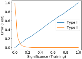
The type I error is easy to calibrate in this method using Eq. (3), since the training and test distributions of in-distribution data should be similar, but the type II error also depends on the unknown distribution of OOD data (Figure 2).
It should be emphasized that, from a hypothesis testing perspective, virtually any function of the input can be used as a statistic, since what we essentially need is the distribution of the statistic under the null hypothesis, or equivalently its value on in-distribution data (as a Monte Carlo approximation). Of course, the power of a statistic depends on the overlap between its distribution on OOD and in-distribution data.
5 Deriving OODDetection Statistics from Invertible Generative Models
Interestingly, some of the generative models that assign high likelihood to OOD data are able to generate fairly plausible images that look like in-distribution images much more than OODs, as also pointed out by Zhang et al. [2020]. This can be explained by noting that observing good images at the model output is the result of a large probability assigned by the model to the 'regions' of the image space where indistribution data lie, but does not necessarily imply that average point-wise likelihood on those data should be high.
To see this with invertible generative models, let us investigate the relation between likelihood and probability under some simplifying assumptions. We consider a certain class C of images (e.g. cats), and assume that any image belonging to this class comes from a bounded region Rc. Now, the probability the model assigns to this class is equal to:
This equation suggests that the probability of observing samples belonging to C (lying in Rc) is related to the integration region as well as the prior density and encoder Jacobian determinant, or equivalently likelihood, over the points in Rc. We note that different combinations of values are possible in theory; for instance, the (average) likelihood may be relatively high but the total probability (Pc) can be low due to the small volume of Rc.
We use Eq. 4 as a heuristic to design statistics aiming at detecting OOD samples, since in principle such samples should come from regions with a small Pc. The terms inside the integral are directly available in formulation of invertible generative models. The region Rc is not well-defined in practice however, particularly because it is difficult to associate an individual sample with a crisp region. Instead of dealing with Rc explicitly, we focus on its volume (Vc) as a quantity that is very informative about the region. But the volume is still an intrinsic characteristic of data distribution that is not directly measurable, unfortunately. For image data, the statistic we found promising in practice as a proxy for region volume is the complexity measure proposed by Serr`a et al. [2020], which is equal to the size of the image when encoded in FLIF compression format 1 . Our intuition is that more complex images (or images with more random noise, in other words)
1 https://flif.info/
come from classes that occupy a higher volume in the space of images. For example, considering single-channel images, blank images have only one degree of freedom, and their corresponding region is in principle a manifold with (virtually) zero volume. In contrast, Gaussian noise images, which have higher complexity and larger compression sizes, are spread over a much larger region. We note that although this statistic is used by Serr`a et al. [2020] for OOD detection as well, the way they look at and use it (in linear combination with log-likelihood) is different from ours.
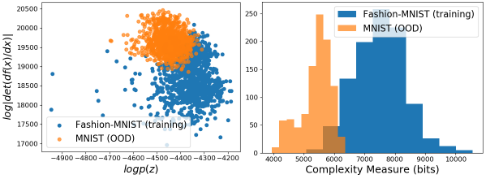
Figure 1 demonstrates an example of the statistics discussed so far on Fashion-MNIST versus MNIST images with iResNet model. The prior density values are almost in the same range for the majority of in-distribution (blue points) and OOD samples (orange) here, but many OODs have relatively large log-determinant values, which gives them higher likelihoods. However, the histogram shows that indistribution data are considerably more complex on average, and thus should occupy a larger volume. This explains how the generative model can assign higher probability to the (region of) in-distribution images. We also note here the two datasets are separated fairly well in the space of log p(z) vs. log-determinant as well as complexity.
It would be very favorable to avoid the Jacobian determinant term, due to its potentially high computational cost. Fortunately, as discussed in the previous section, we are quite free in choosing our statistics in the framework of hypothesis testing, and can make use of other relevant functions, and particularly other functions of the Jacobian matrix. In practice, we have used a function of the Jacobian column sum as a statistic (see the next section), which is much faster to compute than determinant approximation, and is also easy to implement with automatic differentiation tools.
6 Results
We present the results of our OOD detection framework 2 with the following two combinations of statistics, based on the discussions of sections 4 and 5:
2 The code and supplementary material are available at: https://github.com/aahmadian-liu/ood-likefree-invertible
Where pZ(·) and fθ(·) are the prior density and encoder function of the invertible model as before, CFLIF(x) is the size of the input image x (in bits) after compression by the FLIF library, and J(x) denotes the encoder Jacobian matrix of the model at the input x. The second choice is not limited to image data or any external library unlike the first one, though it showed a lower average performance in the experiments.
We evaluate our OOD detection method and compare it to four related methods: Density of States Estimation (Dos) [Morningstar et al., 2021], one-sample Typicality Test [Nalisnick et al., 2019b], S Score obtained from the sum of loglikelihood and compressed image size [Serr`a et al., 2020], and simple log-likelihood threshold based method (Simple LL), which were all briefly introduced in the previous sections. Only the results of DoS with OSVM (and not with KDE) are compared here, since we have used an OSVM as well. The generative models employed in all of the methods are iResNet, ResFlow, and Glow. The performance results in terms of the Area Under ROC curve (AUROC) are given in Table 1 . We have experimented on some of the image dataset pairs which are common in the literature of OOD detection, such as MNIST vs. Fashion-MNIST, and CIFAR10 vs. SVHN. We also include the flipped OOD dataset, that is the horizontal (H) and vertical (V) flipped instances of the test images.
Before feeding the statistics to the OSVM, they are normalized, and PCA is used to remove possible linear correlations. We used the publicly available pretrained models for ResFlow and Glow 3 , but had to train the iResNet ourselves (training details in appendix A). Despite of having Din in Eq. 2, in practice the OSVM is trained on another small partition of the in-distribution data, to reduce the risk of overfitting and training cost. More specifically, the generative model is (or has been) trained on the entire standard training partition of the in-distribution data; the OSVM model is trained on 3000 random samples from the standard test partition of the in-distribution data, and is tested on 3000 different random samples from the test partition of this dataset in addition to 3000 random samples from the OOD dataset. All of the other compared methods have been evaluated on the same test set as well, with the same trained generative model.
The last column in Table 1 clearly shows that the phenomenon of high likelihood OOD samples is present in all of the experimented models, which has led to total failure of conventional likelihood based OOD detection in three cases. The other methods have mitigated this problem to a great extent. However, all the methods have a rather poor performance on most of the difficult dataset pairs, which are the flipped OOD images, and CIFAR10 vs. CIFAR100. This is not surprising since in those cases the in-distribution and OOD images are quite similar in low level features, and discriminating them seems to require a deeper understanding of the content (note that in CIFAR10 vs. CIFAR100, there are several 'close' classes, such as 'dog'/'wolf', and 'bus'/'automobile'). By looking at the samples generated by our models, we realize that they are often not good enough
3 https://github.com/rtqichen/residual-flows, https://github.com/y0ast/Glow-PyTorch at simulating the details which give a 'precise' semantics to the image (appendix E). Hence, we conjecture that the performance bottleneck in these examples is the quality of the generative models, and not the OOD detection framework itself.
The results suggest that our method is generally competitive with the compared ones. Our first setting has the best performance on 5 dataset pairs (though with a slight improvement over the second-best method), and is outperformed by another method only on 2 pairs (FashionMNIST vs. Flip-V, and CIFAR10 vs. Flip-V with ResFlow). In the cases where our method does not rank first, the maximum AUROC difference with the best method is 0.04 and 0.06 for our first and second settings respectively.
Despite of the close performances, the main advantage of our method is its lower computational cost for the invertible models which do not have a closed form Jacobian logdeterminant term. The iResNet and ResFlowmodels approximate this term via a truncated power series and stochastic trace estimator, which is the main bottleneck in computing the log-likelihood required by all the other compared methods (the settings for this approximation in our experiments can be found in appendix B). In Table 2, we have shown the empirical values of the time it takes to compute the log-likelihood (log-determinant term) as well as our Jacobian based statistic (T3) with each of the models. The complexity based statistic (T2) is computed by a fast image compression software (FLIF toolbox), and its computation time is usually small compared to determinant approximation, although the exact time is platform dependent, as it uses a third-party library (around 13ms per image on an Intel Core-i7 laptop with Linux). The conclusion from performance and time results is that substituting log-likelihood with our suggested statistics can hugely speed up the process for some models, without a big decay (if any) in OOD detection performance. The time advantage disappears for Glow, since its log-likelihood does not require approximation. However, it is worth noting that basically Glow has a less flexible network architecture than iResNet/ResFlow , which in practice can hurt the discriminative performance [Behrmann et al., 2019] as well as resulting in larger models (this can be seen by comparing the number of model parameters between the last two rows of Table 2).
Figure 2 gives an instance of type I and II test error curves of our method for Fashion-MNIST vs. MNIST using iResNet. We note that the type I error vs. significance level is close to the identity line, which verifies that training and test statistics of in-distribution data come from the same distribution.
6.1 Ablation Study
We have also investigated other combinations of the introduced statistics in addition to the reported results. Particularly, it was necessary to see if our T2 and T3 statistics provide any additional useful information in practice when added to the log-prior density (T1). We found that adding one of T2 or T3 is often beneficial, but adding both of them is likely to cause slight overfitting. Table 3 gives an instance of the outcomes on CIFAR-10 vs. SVHN with Glow.
| Model / Datasets | Our (T1, T2) | Our (T1, T3) | DoS | S Score | Typicality Test | Simple LL |
|---|---|---|---|---|---|---|
| iResNet trained on MNIST | ||||||
| Fashion-MNIST | 0.99 | 0.99 | 0.99 | 0.97 | 0.99 | 0.99 |
| Uniform Noise | 0.99 | 0.99 | 0.99 | 0.99 | 0.99 | 0.99 |
| Flip-V | 0.57 | 0.56 | 0.56 | 0.54 | 0.49 | 0.51 |
| Flip-H | 0.53 | 0.52 | 0.51 | 0.52 | 0.49 | 0.49 |
| iResNet trained on Fashion-MNIST | ||||||
| MNIST | 0.96 | 0.89 | 0.88 | 0.95 | 0.85 | 0.07 |
| Flip-V | 0.62 | 0.60 | 0.63 | 0.66 | 0.52 | 0.55 |
| Flip-H | 0.56 | 0.55 | 0.56 | 0.56 | 0.50 | 0.52 |
| ResFlow trained on CIFAR-10 | ||||||
| SVHN | 0.96 | 0.92 | 0.94 | 0.89 | 0.80 | 0.10 |
| CIFAR-100 | 0.56 | 0.56 | 0.56 | 0.48 | 0.55 | 0.51 |
| Flip-V | 0.50 | 0.54 | 0.52 | 0.54 | 0.50 | 0.51 |
| Glow trained on CIFAR-10 | ||||||
| SVHN | 0.96 | 0.91 | 0.95 | 0.88 | 0.82 | 0.09 |
| CIFAR-100 | 0.57 | 0.56 | 0.57 | 0.49 | 0.55 | 0.52 |
| Flip-V | 0.51 | 0.51 | 0.51 | 0.51 | 0.50 | 0.50 |
| Model / Training Data | T3 (ms) | Log-Likelihood Approximation (ms) | #Parameters (×106 ) |
|---|---|---|---|
| iResNet (MNIST) | 3 | 209 | 1.17 |
| ResFlow (CIFAR-10) | 20 | 378 | 25.17 |
| Glow (CIFAR-10) | 18 | N/A | 44.23 |
| T2T3 | ¬T2T3 | T2¬T3 | ¬T2¬T3 | |
|---|---|---|---|---|
| T1 | 0.95 | 0.91 | 0.96 | 0.64 |
| ¬T1 | 0.85 | 0.72 | 0.88 | - |
7 Conclusion
Pitfalls of traditional likelihood based OOD detection were re-emphasized in this paper in different aspects, including empirical failure results with the two recent invertible generative models iResNet and ResFlow. Considering that computing likelihood is quite costly in such models as well, an OOD detection method was proposed that is not dependent on likelihood. This method uses a pretrained invertible model and an image complexity measure to summarize the data points in a very low dimensional representation, assigns scores to them using an OSVM, and then classifies them in a null hypothesis testing fashion. The experiments show that, compared to related works, the proposed method has a competitive or even better performance and/or more favorable computational cost in several cases, depending on the datasets and model.
@inproceedings{ijcai2021p292,
  title     = {Likelihood-free Out-of-Distribution Detection with Invertible Generative Models},
  author    = {Ahmadian, Amirhossein and Lindsten, Fredrik},
  booktitle = {Proceedings of the Thirtieth International Joint Conference on
               Artificial Intelligence, {IJCAI-21}},
  publisher = {International Joint Conferences on Artificial Intelligence Organization},
  editor    = {Zhi-Hua Zhou},
  pages     = {2119--2125},
  year      = {2021},
  month     = {8},
  note      = {Main Track},
  doi       = {10.24963/ijcai.2021/292},
  url       = {https://doi.org/10.24963/ijcai.2021/292},
}
TY - CPAPER TI - Likelihood-free Out-of-Distribution Detection with Invertible Generative Models AU - Ahmadian, Amirhossein AU - Lindsten, Fredrik T2 - Proceedings of the Thirtieth International Joint Conference on Artificial Intelligence, IJCAI-21 PB - International Joint Conferences on Artificial Intelligence Organization PY - 2021 SP - 2119 EP - 2125 DO - 10.24963/ijcai.2021/292 UR - https://doi.org/10.24963/ijcai.2021/292 ER -Copied
Machine-readable versions of this paper, for tools and AI agents:





