Modeling Precomputation In Games Played Under Computational Constraints

1 Introduction

While there is a firm theoretical understanding of how perfectly rational agents should play games in equilibrium, understanding the setting where agents have bounded rationality appears to be more challenging. For example, in theory, an agent playing a mini-max game such as chess always has an optimal move it can make. In practice, it may take a very long time to compute an optimal move, and it can be unclear how a rational agent should (or would) behave when it only has a finite amount of time to decide on a move.

Early work on bounded rationality in game theory was motivated by explaining the behavior of agents playing repeated games of the prisoner's dilemma [Neyman, 1985], [Rubinstein, 1986], where agents with bounded rationality were modeled by finite automata. Related work [Megiddo and Wigderson, 1986] extended this to the case where agents were modeled as Turing machines with a restricted number of internal states. As more general models of computation were explored, relations were drawn to well established complexity classes in theory of computation [Papadimitriou and Yannakakis, 1994]. These included explicit external utility costs for complex strategies [Ben-Sasson et al., 2006],[Halpern and Pass, 2015],[Halpern et al., 2016], or implicit discounting of utility for strategies which take longer to compute [Fortnow and Santhanam, 2010]. Much of this line of work was concerned with whether Nash equilibria still exist in this setting, whether they are computable, and what they look like in limiting cases. For mini-max games in particular, a line of work tries to explain why increasing the mini-max search tree depth (i.e. spending more compute time per move) tends to improve agent performance [Ferreira, 2013]. Under certain models increasing the search depth actually worsens the agent's quality [Beal, 1980], [Nau, 1979], [Pearl, 1980], while subsequent work has proposed alternative models to avoid this pathology. (see e.g. [Luˇstrek et al., 2006]). A drawback of much of the prior work mentioned, which is an indication of the challenge of modelling bounded rationality, is that either the models considered are often inflexible and only apply to toy problems (e.g. finite automata, idealized models for search trees, limiting behavior), or the results themselves are infeasible to compute (e.g. equilibrium is computable, but takes exponential time). In contrast, this paper aims to give a relatively flexible model, where some of its properties can be efficiently computed or approximately analyzed.

Consider an extensive form game played between two players, where each player has a finite amount of total time during the game to make their moves. One simple yet underexplored property of these games in the time-constrained setting is the following: before the game, both players can typically spend a large amount of time practicing and preparing, and this time is typically much larger than the amount of time spent playing the game. During the game, if players encounter situations they have prepared for in advance, they are able to play very strong moves quickly from their preparation memory. Otherwise, they have to use their time-limited budget to compute a new move. This simple structure leads to interesting trade-offs. For example, if player 1 plays very deterministically, it will be easy for player 2 to prepare (precompute) strong moves against player 1 using the much larger compute resources available before the match. On the other hand, if player 1 plays more randomly to try and make the future of the game harder to predict, player 1 necessarily needs to play "optimal" moves less frequently. Modeling just this precomputation trade-off leads to surprisingly rich behavior in time constrained games. For example, in chess (which will be used as a running example throughout the paper), human players often (a) prepare against other players by studying certain opening lines they expect to occur in a game (b) play the first few moves of the game quickly from an "opening book" of memorized moves, and (c) intentionally randomize their strategies to make it harder for their opponent to prepare against them. In contrast, many modern chess engines do not explicitly exhibit some of the behavior described above; for example, they will deterministically play the "best move" found within an allotted time, mirroring the idea that in the computationally unbounded setting, there is always an optimal move to play for a mini-max game like chess. In contrast, this paper will show that in the computationally bounded setting where players can precompute, it is perhaps more useful to think in terms of the "best distribution of moves" to play.

Contributions: We first give a novel and flexible formalism for modeling the precomputation aspect of two player, zero sum, perfect information extensive form games played under time constraints. Next, we give theoretical results establishing the importance of randomness of play in the computationally constrained setting. We show that one can efficiently compute how exploitable a fixed strategy is to precomputation, and the equilibrium precomputation strategy between two players. We then empirically demonstrate how useful precomputation can be in practical contexts, by exploring how susceptible Stockfish is to precomputation as a function of randomization.

2 Definitions

2.1 Background

We consider two-player, zero sum, perfect information extensive form games, where the players alternate in turns. In order to provide maximum flexibility of the model, we use standard terminology for game playing which makes no explicit reference to computational constraints. However, we implicitly think of player policies σi as being implemented by some computationally constrained algorithm (e.g. alpha-beta search), and the game being played under some time limit. We will give some concrete examples shortly.

A two-player game consists of a set of histories H, a subset of terminal histories Z ⊂ H, a utility function u : Z → [0, 1] defined on terminal histories h ∈ Z, finite sets of possible actions A(h) for each history h ∈ H \ Z, and a transition function π which takes as input a history h ∈ H \ Z, an action a ∈ A(h), and returns a unique history h′ = π(h, a).

A behavioral strategy (policy) for player i ∈ {1, 2} consists of a function σi defined on H, where σi(h) ∈ ∆(A(h))1 , i.e. σi maps histories to distributions over actions, where σi(h)(a) is the probability that player i plays action a ∈ A(h) when at history h. A player function P : H → {1, 2, c} indicates which player's turn it is to choose an action at history h. If P(h) = c, then h corresponds to a placeholder chance node (i.e. chance player) and an action a ∈ A(h) is chosen according to a fixed probability distribution σc(h).

For notational reasons, we associate each history h ∈ H with the unique ordered sequence (a1, . . . , ak) of actions which must be played to reach h beginning from the starting history ∅ ∈ H, and we say h has length |h| = k. For i ∈ {1, . . . , k} we denote hi = ai, and denote by h:i the history reached by playing a1, . . . , ai, so in particular we have h:i = π(h:i-1, ai). We say h ∈ H is a prefix of h′ if ∃i s.t. h = h′:i , and we write this as h ≤ h′ . The successor function Succ(h) : H → 2H (here 2H is the power set of H) maps a history h to the set of histories H′ ⊂ H where player P(h) next gets to have a turn. Unless explicitly stated, we will consider games where player 1 and 2 alternate in turns with no chance nodes, i.e. P(h) = 1 if |h| is even, P(h) = 2 otherwise.

1 Here ∆ is the probability simplex.

Given a policy profile σ = (σ1, σ2) for both players, the probability of history h′ occurring when starting from history h ≤ h′ is therefore πσ (h, h′ ) = ∏|h′ |-1 i=|h| σP(h′:i )(h′:i )(h′i+1 ), and 0 when h ̸≤ h′ . We define the probability of history h as πσ (h) = πσ (∅, h). We say that the expected value of the game for player 1 when starting from history h ∈ H is uσ1 (h) := ∑h′∈Z πσ (h, h′ )u(h′ ), and uσ2 (h) := 1 - uσ1 (h) for player 2. The expected value of the game for player 1 is uσ1 := uσ1 (∅).

2.2 Algorithmic Strategies and Precomputation

Precomputation strategies are intended to capture the idea that, before a game, we can study some subset S ⊂ H of game histories and plan in advance what to play for these histories. For example, in the case of chess, we could look at some board positions S ⊂ H, and see which moves a powerful chess engine σpre would recommend in these positions after running for an hour. In the actual game, if we ever end up in a position h ∈ S, we can immediately play σpre(h) from a lookup table (without spending any time computing moves). Otherwise, if h ̸∈ S, we can just play our usual policy σi(h) (where we would need to spend compute time during the game).

Definition 1. Given policies σpre, σi, a (σpre, σi,B) precomputation strategy with memory budget B is a policy ˜σi such that:

1. There exists a memorization set S ⊂ H, where |S| ≤ B and S is prefix closed (i.e. if h ∈ S and h′ < h, P (h′ ) = P(h) =⇒ h′ ∈ S).
2. h ∈ S =⇒ ˜σi(h) = σpre(h).
3. h ̸∈ S =⇒ ˜σi(h) = σi(h).

For convenience, we will always think of modeling policies σpre as taking 0 time per move. One justification for considering prefix closed memorization sets is that if a player chooses to memorize history h ∈ H, it is natural for them to have also considered the histories h′ < h leading up to h. We now consider the following meta-game: before a match between player 1 and player 2, which takes place in a timeconstrained setting, each player i can spend time preparing for the match by specially choosing a prefix-closed subset of histories S ⊂ H, and constructing a precomputation strategy ˜σi which plays strong moves according to some policy σpre when in this set. We assume that there is some limiting factor on how many moves each player can memorize for a particular game. In practice, this may be enforced by e.g. a maximum memory budget B, or some limited capacity to memorize moves. We model this by penalizing each player by a linear factor depending on the size of the memorization set of their precomputation strategy. The theory in Section 3 is relatively robust to other choices of penalty functions, but we found the linear penalty led to the most efficient algorithms in Section 4. 2 For more concrete intuition of the formalism one can consider chess: a player can specially prepare a list of opening moves before a tournament, but their capacity to memorize chess lines for a particular match is limited, and their choice invariably depends on the opening move choices prepared for by their opponent as well. This results in an evolving "meta game" of the best opening lines to play.

Definition 2. (The meta-precomputation game) Let Pre(σpre, σi) denote the set of all (σpre, σi, K) precomputation strategies for all K ∈ N, and denote ∆(Pre(σpre, σi)) by the set of all mixed strategies on Pre(σpre, σi). For ˜σ ∈ Pre(σpre, σi), let |˜σ| denote the size of the memorization set used by precomputation strategy ˜σ. Consider a meta-game where each player i instantaneously chooses a mixed precomputation strategy ∆˜σi ∈ ∆(Pre(σpre, σi)), and the outcome utility of the game is

And likewise ˜u2 = 1 - ˜u1. For λ1, λ2 ∈ R+, ∆˜σi ∈ ∆(Pre(σi, σpre)) for i ∈ {1, 2} is an ϵ-Nash equilibrium if

When this is an ϵ = 0 Nash equilibrium, we omit the ϵ and say that vNash = ˜u(∆˜σ1,∆˜σ2) is a Nash equilibrium value of the game.

2.3 Examples

We now give two explicit examples of how we might model games with computational constraints in this framework:

Example 1. (Chess with a time limit per move): Suppose we are playing chess, so h ∈ H corresponds to the prior moves made by each player, A(h) contains all legal moves for player P(h) in state h, and u1(z) = 1 if black is checkmated for z ∈ Z, 0 if white is checkmated by black, and 12 for a draw. We think of σ1, σ2 as chess playing algorithms which each have 1 second per move (concretely, σ1, σ2 = Stockfish(1), Stockfish 3 with a time limit of 1 second per move). If ˜σ1 is a (σpre, σ1,B) precomputation strategy for white with memorization set S, and σpre is a chess playing algorithm which spends 1 hour precomputing per move (concretely, Stockfish(3600)), then when h ∈ S, ˜σ1(h) plays Stockfish(3600)(h) instantaneously; otherwise ˜σ1(h) runs Stockfish(1) on board state h.

2 However, one can still find polynomial time algorithms for other natural penalty functions such as a hard limit on the memorization set size.

3 Stockfish is a popular open source chess playing algorithm.

Example 2. (Chess with a total time limit per game): Consider the previous example, except that instead of having a time limit per move, we now have a time limit of 1 hour for the entire game. Move histories h ∈ H are now augmented to include the time each player took to make their corresponding moves, and the terminal set Z now includes states where players have run out of time (in which case the opposing player wins).

Note that allowing the time an algorithm σ1 takes to depend on the entire history of moves h (instead of just the chess board state) allows us to capture the behavior of algorithms whose computation depends on what they computed in the past; for example, chess playing algorithms often keep a lookup table of moves and positions they have considered during prior moves, in order to speed up future computations.

3 When Do Good Precomputation Strategies Exist?

In this section, we will study how susceptible a fixed policy σi is to precomputation as a function of the randomness of the policy. For simplicity, we will make the definitions from the perspective of player 1 (but the analogous statements hold for player 2). Without loss of generality, we assume that ∀h ∈ Z, P(h) = 1, i.e. the game always ends on player 1's turn. We can do this by adding a sentinel history to every terminal state where this is not the case.

To relate precomputation strategies to randomness of play, we show how to explicitly construct a precomputation strategy whose size depends on how randomly σ2 plays with respect to σpre. This construction then serves as a lower bound on the quality of the best precomputation strategy. The first key observation we make is the following: suppose the game reaches a state h ∈ H such that player 1 now has significant advantage against player 2. Then it should be the case that player 1 can play their normal strategy σ1 against σ2, without any precomputation, and convert this game to a win. Therefore, one way of constructing a precomputation strategy is the following: have player 1 play precomputed moves from σpre against σ2 until a significant advantage (of value v) is gained, and then continue to play normal moves from σ1 afterwards. If σpre is a much stronger policy than σ2, then we expect to not need to play too many moves until an advantage is reached. We can make this observation more concrete by considering the domain of chess: player 1 can play very strong memorized chess engine moves until player 1 has a substantial advantage (e.g. has more pieces on the board than player 2). Player 1 can then play normally to convert this advantage to a win. We formalize this idea with the following definition:

Definition 3. Given policy profile σ = (σ1, σ2), a policy σpre and v ∈ [0, 1], the set histories where player 1 first gets an advantage ≥ v is

We define a distribution S σ,σpre (v) on Sσ (v) via

where the normalizing constant

is the probability of reaching any h ∈ Sσ (v) when σpre plays against σ2.

Example 3. For intuition, if σpre is a much stronger policy than σ2, we expect Pnorm(v) to be close to 1. In the running example of chess, if σpre = Stockfish(1000) and σ1, σ2 = Stockfish(1), we have Pnorm(v) ≥ P [Stockfish(1000) as white checkmates Stockfish(1) as black] for all v ≤ 1, because uσ1,σ2 1 (h) = 1 in every terminal history h where white has checkmated black.

We now observe that if the entropy H(S σ,σpre (v)) of the distribution S σ,σpre (v) is small, then we do not need to memorize too many states to construct the precomputation strategy which memorizes moves until an advantage v is reached. Since we get a value of at least v whenever we end up in h ∈ Sσ (v), we expect a utility of approximately vPnorm(v). We can quantify this observation with the following Theorem:

Theorem 1. Given σ = (σ1, σ2) and a policy σpre, suppose that the maximum number of moves per game is L := maxh∈H |h|. Then ∀v ∈ [0, 1], ϵ ∈ (0, 1), there exists a (σpre, σ1, L(1 - ϵ)eH(S σ,σpre (v))/ϵ ) precomputation strategy ˜σ1 for player 1 such that

where H is the (base e) entropy of the distribution S σ,σpre (v).

For any fixed v ∈ [0, 1], ϵ ∈ (0, 1), Theorem 1 therefore gives us a lower bound on how exploitable a policy σ2 is to precomputation. As expected, there is a direct trade-off between the size of the precomputation set required to exploit σ2, and how randomly σ2 plays against some fixed policy σpre.

We now make the following observation: suppose that ∆˜σ∗ 2 is a Nash equilibrium strategy for player 2 in the metaprecomputation game. If this equilibrium has a favourable equilibrium value for player 2, then it follows from Theorem 1 that S σ,σpre (v′ ) must have high entropy. For the sake of contradiction, suppose that this were not the case: it would then be possible to construct a small precomputation strategy for player 1 which performs well against ∆˜σ∗ 2 but has low precomputation penalty, contradicting the assumption that ∆˜σ∗ 2 has a favourable equilibrium value for player 2. By following this proof by contradiction logic precisely, we obtain the following Theorem. We simplify the statement by considering the case where σpre always wins against ∆˜σ∗ 2 in the original game.

Theorem2. Suppose ∆˜σ∗ 2 is a Nash equilibrium strategy for player 2 with value v in the meta-precomputation game. Suppose that u(σpre,∆˜σ∗ 2 ) 1 = 1, 4 the maximum number of moves in the game is L, and that the precomputation penalty term for player 1 is λ1 > 0. Then ∀v′ ∈ (v + 0.01, 1), we have that

For any fixed v′ ∈ (v+0.01, 1), Theorem 2 therefore quantifies a lower bound on how randomly equilibrium policies play in the precomputation model. The bound tells us that the better the strategy ∆˜σ∗ 2 is for player 2 (the smaller the equilibrium value v is), the more randomly player 2 must play. In contrast to e.g. mini-max games in the computationally unbounded setting where optimal strategies are deterministic, optimal strategies in this model are inherently randomized.

4 Efficiently Finding Precomputation Strategies And Their Equilibria

Suppose we are given oracle access to algorithmic strategies σ1, σ2, σpre. Concretely, we could have σ1, σ2, σpre = Stockfish with different time per move settings. We might believe there is a good precomputation strategy for σ1 against σ2, but it is perhaps unclear how to find such a strategy. Suppose ˜σ1 is an optimal precomputation strategy for player 1 against σ2, with memorization set S. The first observation is that we can assume h ∈ S =⇒ π(σpre,σ2) (h) ≥ λ1; otherwise, player 1 could strictly increase ˜u(˜σ1,σ2) 1 by removing h and any descendants of h from S. This is because the cost of including h and any descendants of h in S is at least λ1, but the gain in utility from any histories which pass through h when precomputing up to h is at most π(σpre,σ2) (h). The second observation is that we can conclude |S| ≤ L+1 λ1 from the following Lemma:

Lemma 1. |{h ∈ H : πσ1,σ2 (h) ≥ p}| ≤ L+1 p , where σ1, σ2 are any policies and the maximum history length of the game is L := maxh∈H |h|.

Thus finding the optimal precomputation strategy for player 1 against σ2 is equivalent to finding the optimal subtree (memorization set) contained within a bounding tree of size L+1 λ1 to memorize. By using standard Chernoff bounds to sample the value of the game at the leaves of this bounding tree, we can compute the optimal subtree with standard dynamic programming techniques. The following Theorem makes these ideas precise, and the detailed algorithm (Algorithm 1) can be found in the technical appendix.

4 i.e. σpre always beats ∆˜σ∗ 2 in the original game, where we implicitly associate the mixed strategy ∆˜σ∗ 2 with a corresponding behavior strategy in the original game by Kuhn's theorem.

Theorem 3. For any ϵ, δ > 0, and precomputation penalty factor λ1 > 0 for player 1, suppose we are given a policy profile σ = (σ1, σ2) and a policy σpre as constant-time oracles. Suppose further that ∃˜σ1 ∈ Pre(σpre, σ1) such that ˜u(˜σ1,σ2) 1 ≥ v. Then with probability at least 1- δ, Algorithm 1 will return a ˜σ′1 ∈ Pre(σpre, σ1) such that ˜u(˜σ′1 ,σ2) 1 ≥ v-ϵ. Moreover, Algorithm 1 runs in time O (A2 L2 λ1ϵ2 ln( A2L λ1 )), where L = maxh∈H |h| and A = maxh∈H |A(h)|.

4.1 Computing Equilibria

In the previous setting, we imagined the opposing player as fixed, while the precomputing player optimizes the best set of game states to memorize in order to exploit the opposing player. In reality, the opposing player reacts to this precomputation by preparing their own lines of play in anticipation to counter this precomputation. In this subsection we will show how an ϵ-Nash equilibrium for the meta-precomputation game can be efficiently found, by reducing the problem to a form which can be solved by the well-studied method of Counter Factual Regret Minimization (CFR) [Zinkevich et al., 2007]. To compute an equilibrium of the meta precomputation game, we first observe (similar to the previous subsection) that we can ignore low probability histories h ∈ H where the possible gain in utility of precomputing at h, regardless of the opposing player's strategy, is always upper bounded by the precomputation penalty λi. For example, player 2 only has an incentive to precompute on the set W2 = {h ∈ H| sup∆˜σ1∈∆Pre(σpre,σ1) π∆˜σ1,σpre (h) ≥ λ2}. If we denote the set of high probability histories by W, then we can bound the size of W by |W| ≤ O (A2 (L+2)2 ( 1 λ1 + 1 λ2 )) (Lemma 3 in technical appendix).

The second observation is that the meta-precomputation game G can be viewed as an equivalent extensive form game G′ with imperfect information and perfect recall. At each game state h ∈ H, we can imagine that instead of players choosing a distribution of actions in A(h) to play, they choose whether to play an action from distribution σpre(h) (i.e. continue precomputing) or distribution σi(h) (stop precomputing); however, if a player chooses to play from distribution σpre(h), they must pay a cost of λi corresponding to the precomputation penalty. We must re-weight this penalty so that it is not discounted by the probability of reaching board state h. Players cannot observe whether their opponent chose to play from distribution σpre(h) or σi(h), but they do see the action which was sampled from the distribution their opponent chose. The memorization set for a precomputation strategy then naturally corresponds to the set of histories where a player chooses to play from distribution σpre(h), and so there is a bijective correspondence between pure strategies in game G, and pure strategies in game G′ . Using the equivalence between behavior strategies and mixed strategies for extensive form games with perfect recall (Kuhn's Theorem), we then get an equivalence between behavior strategies in game G′ , and mixed strategies in game G′ . The precise definition of G′ , and a proof of its equivalence, can be found in the supporting technical appendix (Lemma 4). Thus if we can find an

ϵ-Nash equilibrium of behavior strategies in game G′ , we can find an ϵ-Nash equilibrium of mixed strategies for the metaprecomputation game. Moreover, finding an ϵ-Nash equilibrium for behavior strategies for this new game can be solved efficiently by CFR if we apply previous insights. In particular, we remove low probability histories H \ W from the game, and estimate the value of terminal histories with random roll-outs. The following theorem makes these details precise, and the algorithm (Algorithm 2) can be found in the technical appendix.

Theorem 4. For any ϵ > 0, δ > 0 and precomputation penalty factors λ1, λ2 > 0, suppose we are given a policy profile σ = (σ1, σ2) and a policy σpre as constant-time oracles. Then Algorithm 2 returns an ϵ-Nash equilibrium to the meta-precomputation game with probability at least 1 - δ. Moreover, the total number of CFR iterations is bounded by T = O ( |W|2 ϵ2 ), and the total runtime is bounded by

While these bounds show that in theory one can approximate the Nash equilibrium in polynomial time, in practice it is possible that the equilibrium can be reached after fewer than T = O ( |W|2 ϵ2 ) iterations of CFR. In particular, at iteration T ′ < T , one can use Theorem 3 to verify whether the ϵ-Nash equilibrium condition holds by computing the optimal precomputation strategy value against the current opponent strategy. One can use different variants of CFR which are designed to converge faster in practice depending on the specific structure of the game in question.

5 Experiments

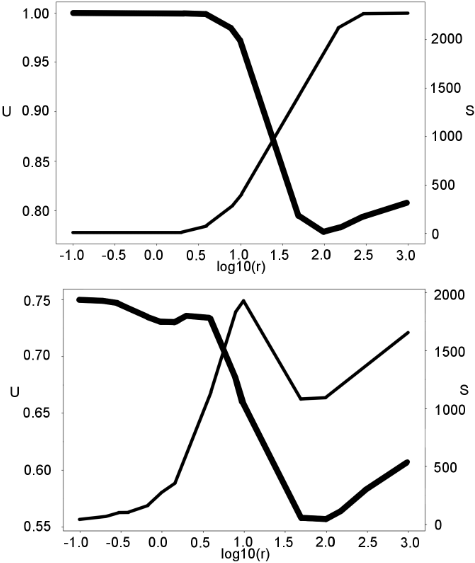
While numerically evaluating CFR to compute equilibria in games is well-studied, finding the correct heuristic variant of CFR to make Algorithm 2 converge quickly for a particular game in practice is a research question on its own, and beyond the scope of this paper. However, the susceptibility of real-world strategies to precomputation, and how useful precomputation can be as a function of the randomness of an opposing strategy, is both relatively unexplored and also feasible to compute in practice without further optimization. We therefore choose to focus on this aspect, and propose an experiment to numerically explore the popular chess engine Stockfish's susceptibility to precomputation using Algorithm 1. Specifically, we choose σpre to be Stockfish with 50ms per move, while σ1 and σ2 play as Stockfish with 10ms per move. For example, Algorithm 1 will transform white=Stockfish(10ms) into a new algorithm white=Stockfish'(10ms), which still takes at most 10ms per move, uses slightly more memory, and performs substantially better against black=Stockfish(10ms) if black does not sufficiently randomize. In particular, we explore how varying the randomness of the policy affects its susceptibility to precomputation. To do this, we introduce a randomness parameter r, and have a policy play more randomly as r increases. As r → 0, σi will play only the best moves found by Stockfish in the required time period. As r →∞, σi will play uniformally between available moves. If player i is the fixed opponent, we set σi(h) = Softmax(Stockfish(h)/r), where Softmax is the softmax function and Stockfish(h) returns a vector of the center pawn (cp) scores of available moves. 5 First we fix the default policies for white (σ1,σpre with r = 10-6 ), and vary r for black (σ2), computing the optimal precomputation value against black for each level of randomness. Then we repeat the experiment for black precomputing against white. We set λ1 = λ2 = 10-5 in these experiments, and plot the precomputed strategy utility (without precomputation penalty) and memorization set size for varying levels of randomness. In order to keep the computation requirements modest, only the top K = 2 moves of the Stockfish engine were considered at each board position. Instead of sampling the game value, a conservative cp bound was used to approximate when either player had a decisive advantage. Further experimentation details can be found in the appendix, and the full code and technical appendix can be found on Github. 6

We see from the results that when either white or black is precomputing, precomputation is particularly effective when the opposition plays predictably (r is small). As the randomness parameter increases, precomputation effectiveness decreases, and more states need to be memorized (the precomputation set size increases). In both plots, there is a transition point at r = 100 (corresponding to one center pawn) where the gain in playing more randomly against precomputation is offset by the loss in playing suboptimally. This suggests an interesting trade-off between playing too predictably and playing the perceived best moves available.

Note that white is able to achieve generally higher precomputation values against black. This can be explained by two observations. The first is that white is generally considered to have an advantage against black, and so Stockfish with 50ms as black does not always win against Stockfish with 10ms as white. The second is that black moves second, which means that black must remember more move variations than white to get to the same precomputation game depth in the game tree. This suggests that the first moving player has an inherent advantage when it comes to precomputation.

6 Conclusion

An unsolved problem in computer science is understanding how computationally bounded agents play games. We contribute to the understanding of this problem by presenting a novel formalism for modeling the precomputation aspect of computationally constrained agents, and show that in contrast to the computationally unconstrained setting, randomization plays an essential role for constructing effective strategies. This result is perhaps in opposition to the conventional heuristic of (deterministically) playing the strongest move found

5 A center pawn score of 100 corresponds to having an advantage of one center pawn.

6 https://github.com/Thomas-Orton/chess-precomputation.

.

within the available time period. Moreover, we showed that optimal strategies in this model can be computed efficiently, and presented empirical results which suggest that precomputation strategies are practically useful in real-world time constrained games such as chess. Our model is flexible, and is essentially equivalent to charging a player depending on which strategy (σi or σpre) they play from in each history. However, the model also has a fundamental structure in connection to the following question in computational complexity theory. Consider a game where there is a time limit of 1 second per move. Informally speaking, suppose we believe there is an algorithm σ1 which achieves value at least v against any other algorithm σ2 which also takes 1 second per move (whether such a σ1 exists is a highly non-trivial problem). 7 Because a precomputation strategy ˜σ2 ∈ Pre(σpre, σ2) takes no more time than one second per move, it follows that σ1 must also have value at least v against ˜σ2, i.e. σ1 must be robust against other algorithms hard-coding constants into their strategy and having non-uniform advice. Exploring this relationship in detail is an area for future work, but the observations about randomness being essential for competitive play are expected to carry over.

7 Here we are informally ignoring the details of program size.