
GraphReach: Position-Aware Graph Neural Network using Reachability Estimations
Proceedings of the Thirtieth International Joint Conference on Artificial Intelligence. Main Track. Pages 1527-1533.
https://doi.org/10.24963/ijcai.2021/211
Keywords
- Data Mining: Mining Graphs, Semi Structured Data, Complex Data
Abstract
Majority of the existing graph neural networks(GNN) learn node embeddings that encode their local neighborhoods but not their positions. Consequently, two nodes that are vastly distant but located in similar local neighborhoods map to similar embeddings in those networks. This limitation prevents accurate performance in predictive tasks that rely on position information. In this paper, we develop GRAPHREACH , a position-aware inductive GNN that captures the global positions of nodes through reachability estimations with respect to a set of anchor nodes. The anchors are strategically selected so that reachability estimations across all the nodes are maximized. We show that this combinatorial anchor selection problem is NP-hard and, consequently, develop a greedy (1−1/e) approximation heuristic. Empirical evaluation against state-of-the-art GNN architectures reveal that GRAPHREACH provides up to 40% relative improvement in accuracy. In addition, it is more robust to adversarial attacks.
- [Brin and Page, 1998] Sergey Brin and Lawrence Page. The anatomy of a large-scale hypertextual web search engine. Computer Networks, 30:107-117, 1998.
- [Chang et al., 2020] Heng Chang, Yu Rong, Tingyang Xu, Wenbing Huang, Honglei Zhang, Peng Cui, Wenwu Zhu, and Junzhou Huang. A restricted black-box adversarial framework towards attacking graph embedding models. In AAAI, pages 3389-3396, 2020.
- [Goyal et al., 2020] Nikhil Goyal, Harsh Vardhan Jain, and Sayan Ranu. Graphgen: A scalable approach to domain- agnostic labeled graph generation. In Proceedings of The Web Conference 2020, pages 1253-1263, 2020.
- [Grover and Leskovec, 2016] Aditya Grover and Jure Leskovec. node2vec: Scalable feature learning for networks. In ACM SIGKDD, pages 855-864, 2016.
- [Gulyás et al., 2018] András Gulyás, Zalán Heszberger, József Bíró, János Tapolcai, Attila Csoma, István Pelle, Attila Kőrösi, Dávid Klajbár, Valentina Halasi, Gábor Rétvári, and Márton Novák. A dataset on human navi- gation strategies in foreign networked systems. Scientific Data, 5, 03 2018.
- [Hamilton et al., 2017] Will Hamilton, Zhitao Ying, and Jure Leskovec. Inductive representation learning on large graphs. In NIPS 2017, pages 1024-1034, 2017.
- [Kipf and Welling, 2017] Thomas N. Kipf and Max Welling. Semi-supervised classification with graph convolutional networks. In 5th ICLR, 2017.
- [Li et al., 2020] Jia Li, Honglei Zhang, Zhichao Han, Yu Rong, Hong Cheng, and Junzhou Huang. Adversar- ial attack on community detection by hiding individuals. In WWW 2020, page 917-927, 2020. [London, 2017] Transport London. Rolling Origin and Des- tination Survey, 2017.
- [Manchanda et al., 2020] Sahil Manchanda, Akash Mittal, Anuj Dhawan, Sourav Medya, Sayan Ranu, and Ambuj Singh. GCOMB: Learning budget-constrained combina- torial algorithms over billion-sized graphs. Advances in Neural Information Processing Systems, 33, 2020.
- [Nemhauser et al., 1978] George Lann Nemhauser, Lau- rence Alexander Wolsey, and Marshall Latham Fisher. An analysis of approximations for maximizing submodular set functions-I. Mathematical Programming, 14(1):265-294, 1978.
- [Pan et al., 2004] Jia-Yu Pan, Hyung-Jeong Yang, Christos Faloutsos, and Pinar Duygulu. Automatic multimedia cross-modal correlation discovery. In ACM SIGKDD, pages 653-658, 2004.
- [Perozzi et al., 2014] Bryan Perozzi, Rami Al-Rfou, and Steven Skiena. DeepWalk: Online learning of social rep- resentations. In ACM SIGKDD, pages 701-710, 2014.
- [Samet, 2006] Hanan Samet. Foundations of multidimen- sional and metric data structures. Academic Press, 2006.
- [TransStat, 2016] RITA TransStat. Origin and Destination Survey database (DB1B), 2016.
- [Velickovic et al., 2018] Petar Velickovic, Guillem Cucurull, Arantxa Casanova, Adriana Romero, Pietro Liò, and Yoshua Bengio. Graph attention networks. In 6th ICLR, 2018.
- [Wadhwa et al., 2019] Sarisht Wadhwa, Anagh Prasad, Sayan Ranu, Amitabha Bagchi, and Srikanta Bedathur. Efficiently answering regular simple path queries on large labeled networks. In ICMD, pages 1463-1480, 2019.
- [West and Leskovec, 2012] Robert West and Jure Leskovec. Human wayfinding in information networks. In WWW, page 619-628, 2012.
- [Xu et al., 2019] Keyulu Xu, Weihua Hu, Jure Leskovec, and Stefanie Jegelka. How powerful are graph neural net- works? In 7th ICLR, 2019.
- [Xu et al., 2020] Chunyan Xu, Zhen Cui, Xiaobin Hong, Tong Zhang, Jian Yang, and Wei Liu. Graph inference learning for semi-supervised classification. In 8th ICLR, 2020.
- [You et al., 2019] Jiaxuan You, Rex Ying, and Jure Leskovec. Position-aware graph neural networks. In ICML, pages 7134-7143, 2019.
- [Zhu et al., 2020] Jiong Zhu, Yujun Yan, Lingxiao Zhao, Mark Heimann, Leman Akoglu, and Danai Koutra. Be- yond homophily in graph neural networks: Current limita- tions and effective designs. In NeurIPS, 2020.
References were extracted automatically from the PDF and may contain errors.
Full text extracted automatically from the PDF; figures, tables and equations may differ. The PDF is the version of record.
1 Introduction and RelatedWork
Learning feature-space node embeddings through graph neural networks (GNN) has received much success in tasks such as node classification, link prediction, graph generation, learning combinatorial algorithms, etc. [Hamilton et al., 2017; Kipf and Welling, 2017; Velickovic et al., 2018; Goyal et al., 2020; Manchanda et al., 2020]. GNNs learn node embeddings by first collecting structural and attribute information from the neighborhood of a node and then encoding this information into a feature vector via non-linear transformation and aggregation functions. This allows GNNs to generalize to unseen nodes, i.e., nodes that were not present during the training phase. This inductive learning capability of GNNs is one of the key reasons behind their popularity.
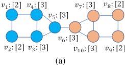
Due to reliance on only the neighborhood information, most GNN architectures fail to distinguish nodes that are located in different parts of the graph, but have similar neighborhoods. In the extreme case, if two nodes are located in topologically isomorphic neighborhoods, their learned embeddings are identical. To elaborate, consider nodes v1 and v8 in Fig. 1a. The two nodes belong to two different class labels (node color). However, since their 2-hop neighborhoods are isomorphic to each other, their learned embeddings in a 2-layer Graph Convolutional Network (GCN) are identical, despite the fact that they are far away in the graph. Hence, the GCN will be incapable of correctly predicting that v1 and v8 belong to different class labels. Consequently, for predictive tasks that rely on position of a node with respect to the graph, the performance suffers. While node embedding methods such as DeepWalk [Perozzi et al., 2014] and Node2Vec [Grover and Leskovec, 2016] do learn position information, they are transductive in nature, i.e., they fail to generalize to unseen nodes. In addition, they cannot encode attribute information. Our goal, therefore, is to design a GNN that is inductive, captures both position as well as node attribute information in the embeddings, and overcomes the problem of automorphism leading to identical embeddings.
We emphasize that we do not claim position information to be more important than the neighborhood structure. Rather, the more appropriate choice depends on the problem being solved and the dataset. For example, if homophily is the main driving factor behind a prediction task, then embeddings based on local neighborhood structure are likely to perform well. On the other hand, to predict whether two nodes belong to the same community, e.g., road networks, gene interaction networks, etc., positional information is more important.
P-GNN [You et al., 2019] is the first work to address the need for an inductive GNN that encodes position information. P-GNN randomly selects a small number of nodes as anchor nodes. It then computes the shortest path distances of all remaining nodes to these anchor nodes, and embeds this information in a low-dimensional space. Thus, two nodes have similar embeddings if their shortest path distances to the anchors are similar. To illustrate, we revisit Fig. 1a, and assume that v7 is an anchor node. Although the 2-hop neighborhoods of v1 and v8 are isomorphic, their shortest path distances to v7 are different and, hence, their embeddings will be different as well. Although P-GNN has shown impressive improvements over existing GNN architectures in link prediction and pairwise node classification, there is scope to improve.
| Symbol | Dimensions | Description |
|---|---|---|
| X = {xv | ∀v ∈ V} Hl = {hlv | ∀v ∈ V} Ml = {Mlv | ∀v ∈ V} WlM alatt Z = {zv | ∀v ∈ V} WZ | n × d n × dhid n×k ×dhid 2 · dhid ×dhid 2 · dhid ×1 n × k dhid × 1 | Original node attributes Feature matrix at layer l Message Tensor at layer l TransformMl Attention vector at layer l Output embeddings TransformsML to Z |
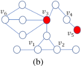
1. Holistic Position Inference: Since P-GNN relies only on shortest path distances to compute embeddings, remaining paths of the graph are ignored. Consequently, two nodes can be incorrectly concluded to be in the same position, even if they are not. Fig. 1b illustrates this aspect. Here, nodes v1, v2, and v6 are all equidistant from the anchors v3 and v5 and consequently, their embeddings would be similar. Note, however, that v6 is located in a different region with several paths of length 2 to v3, whereas v1 and v2 have only one path. Thus, v6 should have a different embedding.
2. Semantics: The assumption of shortest path rarely holds in the real world. This has been shown across varied domains such as Wordmorph [Guly´as et al., 2018], Wikispeedia [West and Leskovec, 2012], metro transportation [London, 2017], flight connections [TransStat, 2016], etc. Instead, many short paths are followed [West and Leskovec, 2012].
3. Robustness to Adversarial Attacks: Relying only on shortest paths also makes P-GNN vulnerable to adversarial attacks. Specifically, adding a small number of critical edges in the graph can significantly alter the shortest path distances for targeted nodes and, hence, their node embeddings.
To overcome these shortcomings, in this paper, we introduce a new position-aware GNN architecture called GRAPHREACH 1 . Our key contributions are as follows:
- GRAPHREACH computes position-aware inductive node embeddings through reachability estimations. Reachability estimations encode the position of a node with respect to all paths in the graph (§2 and §3). This holistic position estimation also ensures that GRAPHREACH is robust to adversarial attacks since a few edge additions or deletions do not substantially alter the reachability likelihoods (§4.5).
- Unlike P-GNN, where anchors are randomly selected, GRAPHREACH strategically selects anchors by framing it as a problem of maximizing reachability along with their attention weights. We show that maximizing reachability is NP-hard, monotone and submodular. We overcome this bottleneck through a greedy hill-climbing algorithm, which provides a (1-1/e) approximation guarantee (§3.2).
- Extensive empirical evaluation across 8 datasets demonstrates a dramatic relative improvement of up to 40% over P-GNN and other state-of-the-art GNN architectures (§4).
1 Appendices are in https://arxiv.org/abs/2008.09657/.
2 ProblemFormulation
We represent a graph as G = (V, E,X,W), where V is the set of nodes vi, with 1 ≤ i ≤ n and E is the set of edges. The attribute set X = {xv1 , · · · , xvn } has a one-to-one correspondence with the node set V where xvi represents the feature vector of node vi ∈ V. Similarly, W has a one-to-one correspondence with E, where wei denotes the edge weights.
A node embedding model is a function f : V → Z that maps the node set V to a d-dimensional vector space Z = {z1, · · · , zn}. Our goal is to learn a position-aware node embedding model [You et al., 2019].
Definition 1 (Position-aware Embedding). A node embedding zv, ∀v ∈ V is position-aware if there exists a function g(·, ·) such that d(vi, vj) = g(zi, zj), where d(vi, vj) is the distance from vi to vj in G.
The distance d(vi, vj) should reflect the quality of all paths between vi and vj wherein, (1) d(vi, vj) is directly proportional to the number of paths between vi and vj, and (2) d(vi, vj) is inversely proportional to the lengths of the paths between vi and vj . We capture these aspects in the form of reachability estimations through random walks. Note that, d(·, ·) is not required to be a metric distance function.
Reachability estimations are similar to PageRank [Brin and Page, 1998] and Random Walk with Restarts [Pan et al., 2004]. To the best of our knowledge, GIL [Xu et al., 2020] is the only other GNN framework that uses the concept of reachability estimations. However, GIL does not use reachability to learn node embeddings. Rather, they are used as additional features along with node embeddings for node classification. Reachability Estimations: In a fixed-length random walk of length lw, we start from an initial node vi, and jump to a neighboring node u through an outgoing edge e = (vi, u) with transition probability p(e) = we/ ∑∀e′∈N(vi) we′ . Here, N(vi) denotes the set of outgoing edges from vi. From node u, the process continues iteratively in the same manner till lw jumps. If there aremany short paths fromvi to vj, there is a high likelihood of reaching vj by a random walk from vi. We utilize this property to define a similarity measure:
Here, nw denotes the number of random walks started from vi, and countk(vi, vj) denotes the number of times random walker visited vj in the kth random walk starting from vi. The similarity function could also weight the nodes according to the order they appear in a random walk (refer to App. A). From s(vi, vj), one may define d(vi, vj) = 1-s(vi, vj ). However, we directly work with similarity s(·, ·) since d(vi, vj) is not explicitly required in our formulation.
3 GRAPHREACH
The symbols and notations used through out this paper are summarized in Table 1. All the matrix and vector notations are denoted in bold letters by convention.
3.1 The Architecture
Algo. 1 outlines the pseudocode and Fig. 2 pictorially depicts the architecture. In addition to hyper-parameters and message
Algorithm 1 GRAPHREACH
Input: Graph G = (V, E,X,W); Anchors {ai}; Message computation function F; Message aggregation function S; Number of layers L; Non-linear function σ
Output: Node embedding zv, ∀v ∈ V
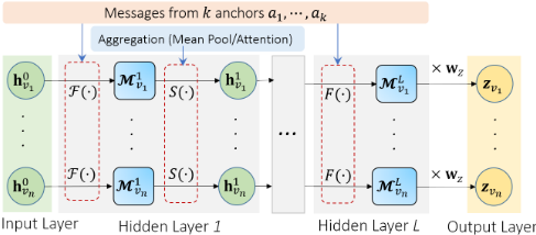
1: h0v ← xv, ∀v ∈ V 2: for l = 1, · · · ,L do 3: for v ∈ V do 4: for i = 1, · · · , k do 5: ̂Mlv[i] ←F(v, ai, hl-1 v , hl-1 ai ) ▷Msg Computation 6: Mlv = (⊕ai∈A ̂Mlv[i])·WlM▷Concatenation: Eq. (5) 7: hlv ← S (Mlv ) ▷ Msg Aggr: Eq. (6) and Eq. (8) 8: return zv ∈ Rk ← σ(MLv .WZ), ∀v ∈ Vpassing functions, the input to Algo. 1 includes the graph and k anchor nodes. The details of the anchor selection procedure are discussed in §3.2. In the initial layer, the embedding of a node v is simply its attribute vector xv (line 1). In each hidden layer, a set of messages, Ml , is computed using the message computing function F(v, a, hlv , hla ) between each node-anchor pair (details in §3.3) (lines 2-6). The componentMlv [i] inMl represents the message received by node v from the ith anchor node. These messages are then aggregated using an aggregation function S (line 7), which we will discuss in detail in §3.4. The aggregated messages thus obtained are propagated to the next layer. In the final layer, the set of messages for each node, i.e.,Mlv , is linearly transformed through a trainable weight matrixWZ (line 8).
3.2 Anchor Selection
Anchors act as our reference points while encoding node positions. It is therefore imperative to select them carefully. Selecting two anchors that are close to each other in the graph is not meaningful since the distance to these anchors from the rest of the nodes would be similar. Ideally, the anchors should be diverse as well as reachable from a large portion of nodes.
Formally, let R be the set of all random walks performed across all nodes in V. We represent the reachability information in the form of a bipartite graph B = (V1, V2, EB). Here, V1 = V2 = V. There is an edge e = (u, v) ∈ EB, u ∈ V1, v ∈ V2 if there exists a walk in R that starts from v and reaches u. The reachability set of a subset of nodes A is:
Our objective is to find the set of k anchors A∗ ⊆ V1, |A∗ | = k, that maximizes reachability. Specifically,
Lemma 1. The maximization problem in Eq. 3, performed on the bipartite graph formed on the reachability set, is NP-hard.
Lemma 2. For any given set of nodes A, f(A) = |ρ(A)| is monotone and submodular.
The proofs are in App. B and App. C respectively.
For monotone and submodular optimization functions, the greedy-hill climbing algorithm provides a (1 - 1/e) approximation guarantee [Nemhauser et al., 1978]. We, thus, follow the same strategy and iteratively add the node that provides highest marginal reachability (Algo. 2 in App. D).
Corollary 1. If set A is the output of Algo. 2 (in App. D), then | ρ(A) |≥ (1-1/e) | A∗ |, where A∗ is the anchor set of size k that maximizes reachability coverage.
PROOF. Follows from Lemma 2.
Modeling Reachability Frequency: The above approach models reachability as a binary occurrence; even if there exists just one walk where v ∈ V2 reaches u ∈ V1, an edge (u, v) is present in B. It does not incorporate the frequency with which u is visited from v. To capture this aspect, we randomly sample X% of the walks from R and form the bipartite graph only on this sampled set. Note that the downsampling does not require the bipartite graph to be fully connected. Algo. 2 (in App. D) is next run to select anchors on this bipartite graph. This process is repeated multiple times by drawing multiple samples of the same size from R and the final anchor set consists of nodes that are selected in the answer sets the highest number of times. In our experiments, we sample 5 subsets with X = 30%.
3.3 Message Computation
The message computation function F (v, a, hlv , hla ) should incorporate both the position information of node v with respect to the anchor set A as well as the node attributes. While node attributes may provide important information that may be useful in the eventual prediction task, position information, in the form of reachability estimations, captures the location of the node in the global context of the graph. To encode these dual needs, F (v, a, hlv , hla ) is defined as follows.
where ‖ denotes concatenation of vectors. The function F takes as input a node v, an anchor a and their respective layer attributes, hlv and hla . It returns a message vector, which is a weighted aggregation of their individual attributes in proportion to their reachability estimations (Eq. 1). Observe that, the reachability estimations are used in both directions to account for an asymmetric distance function.
Due to concatenation, the output message vector is of dimension 2 · dhid, where dhid is dimension of the node embeddings in the hidden layers. To linearly transform the message vector back into Rdhid , we multiply it with a weight vector WlM . The complete global structure information for node v is encompassed in the message matrixMlv (⊕ denotes rowwise stacking of message vectors).
3.4 Message Aggregation
To compute the hidden representation of nodes, messages corresponding to anchors are aggregated for each node. We propose two aggregation schemes.
- Mean Pool (M): In this, a simple mean of the message vectors are taken across anchors.
2. Attention Aggregator (A): In mean pooling, all anchors are given equal weight. Theorizing that the information being preserved can be enhanced by capturing the significance of an anchor with respect to a node, we propose to calculate the significance distribution among anchors for each node. Following the Graph Attention Network (GAT) architecture [Velickovic et al., 2018], we compute attention coefficients of anchors for an anchor-based aggregation. The attention coefficient of the ith anchor ai is computed with trainable weight vector alatt and weight matrixWlatt . For node v, the attention weight with respect to anchor i is
Here, sm denotes the softmax function. As followed in GAT architecture [Velickovic et al., 2018], we use LeakyReLU as the non-linear function σatt (with negative input slope 0.2).
Finally, the messages are aggregated across anchors using these coefficients.
3.5 Hyper-parameters for Reachability Estimation
Reachability information relies on two key random walk parameters: the length lw of each walk, and the total number of walks nw. If lw is too short, then we do not gather information with respect to anchors more than lw-hops away. With nw, we allow the walker to sample enough number of paths so that our reachability estimations are accurate and holistic. We borrow an important theorem from [Wadhwa et al., 2019] to guide our choice of lw and nw.
Theorem 1. [Wadhwa et al., 2019] If there exists a path between two nodes u and v in a graph, with 1-1/n probability the random walker will find the path if the number of random walks conducted, nw, is set to Θ( 3√n2 lnn) with the length of each random walk, lw, being set to the diameter of the graph.
3.6 Complexity Analysis
We conduct nw random walks of length lw for all the n nodes of the graph; this requires O(nw · lw · n) time. For anchor set selection, we sample random walks multiple times and select k anchors using the resulting bipartite graphs formed. The complexity of sampling walks is O(n · nw) while selecting the anchors takes O(k + k · log k) = O(k · log k) operations. Considering that each node communicates with k anchors, there are O(n · k) message computations. The aggregation of messages also requires O(n · k) operations owing to k messages being aggregated for each of the n nodes. The attention aggregator has an additional step devoted to computation of attention coefficients which takes O(n · k) time as well.
| Datasets | #Nodes | #Edges | #Labels | Diameter | #Attributes |
|---|---|---|---|---|---|
| Grid | 400 | 760 | - | 38 | - |
| Communities | 400 | 3.8K | 20 | 9 | - |
| PPI | 56.6K | 818K | - | 8 | 50 |
| Email-Complete | 986 | 16.6K | 42 | 7 | - |
| 920 | 7.8K | 6 | 7 | - | |
| Protein | 43.4K | 81K | 3 | 64 | 29 |
| CoRA | 2.7K | 5.4K | 7 | 19 | 1433 |
| CiteSeer | 3.3K | 4.7K | 6 | 28 | 3703 |
4 Experiments
In this section, we benchmark GRAPHREACH and establish that GRAPHREACH provides up to 40% relative improvement over state-of-the-art GNN architectures. The implementation is available at https://github.com/idea-iitd/GraphReach.
4.1 Experimental Setup
Please refer to App. E for information on reproducibility.
Datasets: We evaluate GRAPHREACH on the datasets listed in Table 2. Further details are available in App. E.
Baselines: We measure and compare the performance of GRAPHREACH with five baselines: (1) P-GNN [You et al., 2019], (2) GCN [Kipf and Welling, 2017], (3) GRAPHSAGE [Hamilton et al., 2017], (4) GAT [Velickovic et al., 2018], and (5) GIN [Xu et al., 2019].
Prediction Tasks: We evaluate GRAPHREACH on the prediction tasks of Link Prediction (LP) and Node Classification (NC) using the Binary Cross Entropy (BCE) loss with logistic activation, and on Pairwise node classification (PNC) using the Negative Log Likelihood (NLL) loss.
Setting: For LP, we evaluate in both inductive and transductive settings, whereas for PNC , only inductive setting is used. Default Parameters and Design Choices: Unless specifically mentioned, we set the number of anchors (k) as log2 n. While our experiments reveal that a smaller number of anchors is sufficient, since P-GNN uses log2 n anchors, we keep it the same. The length of each random walk, lw, is set to graph diameter, and the number of walks nw as 50. We also conducted experiments to analyze how these parameters influence prediction accuracy of GRAPHREACH.
We use Attention aggregation (Eq. 8) and simple random walk counts as the similarity function (Eq. 1) to compare with the baselines. For a fair comparison, values of parameters that are common to GRAPHREACH and other baselines are kept the same. Their exact values are reported in App. E.
4.2 Comparison with Baselines
Pairwise Node Classification (PNC): Table 3a summarizes the performances in PNC. We observe a dramatic performance improvement by GRAPHREACH over all existing GNN architectures. While P-GNN clearly established that encoding global positions of nodes helps in PNC, GRAPHREACH further highlights the need to go beyond shortest paths. Except
| Models | Communities | Email-Complete | Protein | Models | Grid-T | Communities-T | Grid | Communities | PPI | |
|---|---|---|---|---|---|---|---|---|---|---|
| GCN | 0.520±0.025 | 0.515±0.019 | 0.536±0.006 | 0.515±0.002 | GCN | 0.698±0.051 | 0.981±0.004 | 0.456±0.037 | 0.512±0.008 | 0.769±0.002 |
| GRAPHSAGE | 0.514±0.028 | 0.511±0.016 | 0.508±0.004 | 0.520±0.003 | GRAPHSAGE | 0.682±0.050 | 0.978±0.003 | 0.532±0.050 | 0.516±0.010 | 0.803±0.005 |
| GAT | 0.620±0.022 | 0.502±0.015 | 0.511±0.008 | 0.528±0.011 | GAT | 0.704±0.050 | 0.980±0.005 | 0.566±0.052 | 0.618±0.025 | 0.783±0.004 |
| GIN | 0.620±0.102 | 0.545±0.012 | 0.544±0.010 | 0.523±0.002 | GIN | 0.732±0.050 | 0.984±0.005 | 0.499±0.054 | 0.692±0.049 | 0.782±0.010 |
| P-GNN-F | 0.997±0.006 | 0.640±0.037 | 0.630±0.031 | 0.729±0.176 | P-GNN-F | 0.637±0.078 | 0.989±0.003 | 0.694±0.066 | 0.991±0.003 | 0.805±0.003 |
| P-GNN-E | 1.000±0.001 | 0.640±0.029 | 0.637±0.037 | 0.631±0.175 | P-GNN-E | 0.834±0.099 | 0.988±0.003 | 0.940±0.027 | 0.985±0.008 | 0.808±0.003 |
| GRAPHREACH 1.000±0.000 | 0.949±0.009 | 0.935±0.006 | 0.904±0.003 | GRAPHREACH | 0.945±0.021 | 0.990±0.005 | 0.956±0.014 | 0.991±0.003 | 0.810±0.002 | |
(a) Pairwise Node Classification (PNC)
(b) Link Prediction (LP)
| Task | Dataset | GCN | GRAPHSAGE | GAT | GIN | P-GNN | GRAPHREACH | ||||||
|---|---|---|---|---|---|---|---|---|---|---|---|---|---|
| S+T | S | S+T | S | S+T | S | S+T | S | S+T | S | S+T | S | ||
| LP | CoRA | 0.86 | 0.59 | 0.85 | 0.53 | 0.86 | 0.51 | 0.86 | 0.59 | 0.81 | 0.77 | 0.83 | 0.84 |
| LP | CiteSeer | 0.87 | 0.61 | 0.85 | 0.56 | 0.87 | 0.56 | 0.86 | 0.68 | 0.77 | 0.76 | 0.77 | 0.74 |
| PNC | CoRA | 0.98 | 0.50 | 0.96 | 0.50 | 0.98 | 0.51 | 0.98 | 0.52 | 0.86 | 0.59 | 0.96 | 0.77 |
| PNC | CiteSeer | 0.96 | 0.51 | 0.95 | 0.51 | 0.96 | 0.50 | 0.96 | 0.53 | 0.77 | 0.57 | 0.91 | 0.61 |
| NC | CoRA | 0.92 | 0.52 | 0.92 | 0.50 | 0.90 | 0.50 | 0.90 | 0.54 | 0.73 | 0.50 | 0.84 | 0.86 |
| NC | CiteSeer | 0.82 | 0.52 | 0.82 | 0.50 | 0.81 | 0.50 | 0.82 | 0.53 | 0.73 | 0.55 | 0.75 | 0.71 |
Table 4: ROC AUC. ('S' denotes the version containing only the graph structure and 'S+T' denotes structure with node attributes.)
in Communities, the highest accuracy achieved by any of the baselines is 0.73. In sharp contrast, GRAPHREACH pushes the ROC AUC above 0.90, which is a significant ≈ 40% relative improvement, on average, over the state-of-the-art.
Link Prediction (LP): Table 3b presents the results for LP. Consistent with the trend observed in PNC, GRAPHREACH outperforms other GNNs across inductive and transductive settings. P-GNN and GRAPHREACH are significantly better than the rest of the architectures. This clearly indicates that position-aware node embeddings help. GRAPHREACH being better than P-GNN suggests that a holistic approach of encoding position with respect to all paths is necessary.
The second observation from Table 3b is that the performance of position-unaware architectures are noticeably better in transductive setting. Since transductive setting allows unique identification of nodes through one-hot encodings, traditional GNN architectures are able to extract some amount of position information, which helps in the prediction. In contrast, for both P-GNN and GRAPHREACH, one-hot encodings do not impart any noticeable advantage as position information is captured through distances to anchors.
We also compare the time taken by the two best performing models (in App. F). On average, GRAPHREACH is 2.5 times faster than P-GNN owing to its strategic anchor selection.
4.3 Difference fromNeighborhood-based GNNs
We conducted experiments on attributed graph datasets, with and without attributes for prediction tasks. Table 4 presents the results for CoRA and CiteSeer on LP, PNC and NC.
In addition to the network structures, both CoRA and CiteSeer, are also accompanied by binary word vectors characterizing each node. When the word vectors are ignored, the performance of neighborhood-aggregation based GNNs are significantly inferior (≈ 25%) to GRAPHREACH. When supplemented with word vectors, they outperform GRAPHREACH (≈ 10% better). This leads to the following conclusions. (1) Position-aware GNNs are better in utilizing the structural information. (2) Neighborhood-aggregation based GNNs may be better in exploiting the feature distribution in the neighborhood. (This is not always though, e.g., in PPI and Protein, GRAPHREACH is better than the baselines even when attribute information is used as seen in Tables 3a and 3b). (3) The two approaches are complementary in nature and, therefore, good candidates for ensemble learning. To elaborate, neighborhood aggregation based architectures rely on homophily [Zhu et al., 2020]. Consequently, if the node property is a function of neighborhood attribute distribution, then neighborhood aggregation performs well. On the other hand, in LP, even if the local neighborhoods of two distant nodes are isomorphic, this may not enhance their chance of having a link. Rather, the likelihood increases if two nodes have many neighbors in common. When two nodes have common neighbors, their distances to the anchors are also similar, and this positional information leads to improved performance.
4.4 Ablation Study: Mean Pool versus Attention
In the first two rows of Table 5, we compare the performance of GRAPHREACH with Attention (GRAPHREACH-A) and Mean Pool (GRAPHREACH-M) aggregation functions. As clearly evident, the performance is comparable. In mean pool, the message from each anchor is weighted equally, while when an attention layer is used, GRAPHREACH learns an additional importance weight for each anchor to aggregate messages. The comparable performance of Mean Pool with Attention shows that similarity encoded in the message from each anchor is enough to learn meaningful embeddings; the marginal gain from an additional attention layer is minimal. To further substantiate this claim, we alter Eq. 4 to F (v, a, hlv , hla ) = hlv ‖ hla ; i.e, contributions of all anchors are made equal. The variant GRAPHREACH-M- presents the performance with this modification; as evident, there is a massive drop in accuracy. We also evaluate GRAPHREACH using a similarity function variant (in App. F).
4.5 Adversarial Attacks
We assume the standard black-box adversarial setup where the attacker has knowledge of only the graph and can modify it through addition or deletion of edges [Li et al., 2020; Chang et al., 2020]. Let G = (V, E) be the test graph which has a colluding subset of nodes C ⊆ V. The nodes in C can add as many edges as needed among them so that predictions on C are inaccurate. For PNC, we randomly sample 10% nodes from the unseen test graph, and form a clique among these colluding nodes. For LP, we randomly sample 10% of the node pairs from the unseen test graph such that they do
| Models | Communities | Email-Complete | Protein | Models | Grid-T | Communities-T | Grid | Communities | PPI | |
|---|---|---|---|---|---|---|---|---|---|---|
| GR-A | 1.000±0.000 | 0.949±0.009 | 0.935±0.006 | 0.904±0.003 | GR-A | 0.945±0.021 | 0.990±0.005 | 0.956±0.014 | 0.991±0.003 | 0.810±0.002 |
| GR-M | 1.000±0.000 | 0.938±0.017 | 0.945±0.004 | 0.916±0.008 | GR-M | 0.940±0.018 | 0.994±0.003 | 0.931±0.020 | 0.993±0.003 | 0.830±0.004 |
| GR-M- | 0.500±0.000 | 0.500±0.000 | 0.500±0.000 | 0.559±0.007 | GR-M- | 0.542±0.071 | 0.888±0.046 | 0.500±0.000 | 0.500±0.000 | 0.519±0.026 |
1.0
(a) Pairwise Node Classification (PNC)
(b) Link Prediction (LP)

| Dataset | Task | P-GNN | GRAPHREACH | ||||
|---|---|---|---|---|---|---|---|
| Bf | Af | ∆ | Bf | Af | ∆ | ||
| Communities | PNC | 0.92 | 0.82 | 0.10 | 1.00 | 0.98 | 0.02 |
| Communities | LP | 1.00 | 0.89 | 0.11 | 1.00 | 1.00 | 0.00 |
Table 6: Robustness to adversarial attacks. (Bf and Af indicate ROC AUC before and after collusion respectively, while ∆ denotes the change in accuracy due to collusion.)
not have an edge between them. From this set, we select the top-2% of the highest degree nodes and connnect them to the remaining colluding nodes through an edge. This makes the diameter of the colluding group at most 2.
We perform prediction using pre-trained models of both PGNN and GRAPHREACH on the test graph and measure the ROC AUC on the colluding group. This process is repeated with 5 different samples of colluding groups and the mean accuracy is reported. If the model is robust, despite the collusion, its prediction accuracy should not suffer.
As visible in Table 6, the impact on the accuracy of GRAPHREACH is minimal. On the other hand, P-GNN receives more than 10% relative drop in the performance. This result highlights one more advantage of reachability estimations. Since GRAPHREACH incorporates all paths in its position-aware embeddings, causing a significant perturbation in position with respect to all paths in the network is difficult. In case of P-GNN, perturbing shortest paths is relatively easier and hence there is a higher impact on the performance.
4.6 Impact of Parameters
Random Walk Length, lw: Fig. 3a presents the result on three datasets covering both PNC and LP. Results on remaining datasets are provided in App. F. On Communities and Email-Complete, the impact of lw is minimal. However, in Protein, the accuracy saturates at around lw = 40. This is a direct consequence of the property that Protein has a significantly larger diameter of 64 than both Communities and Email-Complete (see Table 2). Recall from our discussion in §3.5 that setting lw to the graph diameter is recommended for ensuring accurate reachability estimations. The trends in Fig. 3a substantiate this theoretical result.
Number of Random Walks, nw: Fig. 3b presents the results. As expected, with higher number of walks, the accuracy initially improves and then saturates. From §3.5, we know that nw should increase with the number of nodes in the graph to ensure accurate reachability estimations. The trend in Fig. 3b is consistent with this result. In App. F, we present the results for this experiment on the remaining datasets.
Number of Anchors and Anchor Selection Strategy: Fig. 3(c-d) present the results. In addition to the default anchor selection strategy, we also evaluate the accuracy obtained when an equal number of anchors are selected randomly. Two key properties emerge from this experiment. First, as the number of anchors increases, the accuracy improves till a saturation point. This is expected since with more anchors we have more reference points to accurately encode node positions. Second, the proposed anchor selection strategy is clearly better than random anchor selection. More importantly, the proposed anchor selection strategy saturates at around 2.5% compared to 5% in random. Recall that the dimension of the final embeddings, i.e., the final layer, is equal to the number of anchors. Consequently, this experiment highlights that high quality embeddings can be obtained within a low-dimensional space. A low dimension is preferred in various tasks such as indexing and querying of multi-dimensional points, due to the adverse impacts of curse-of-dimensionality [Samet, 2006].
5 Conclusions
GNN architectures, despite their impressive success in learning node embeddings, suffer on predictive tasks that rely on positional information. Though P-GNN recognized this need, due to reliance on only shortest paths, the position information captured by P-GNN is not holistic. GRAPHREACH addresses this limitation and builds a different positional model based on reachability estimations to anchors computed strategically through fixed-length random walks. GRAPHREACH achieves a relative improvement of up to 40% over other architectures, while also being robust to adversarial attacks.
@inproceedings{ijcai2021p211,
  title     = {GraphReach: Position-Aware Graph Neural Network using Reachability Estimations},
  author    = {Nishad, Sunil and Agarwal, Shubhangi and Bhattacharya, Arnab and Ranu, Sayan},
  booktitle = {Proceedings of the Thirtieth International Joint Conference on
               Artificial Intelligence, {IJCAI-21}},
  publisher = {International Joint Conferences on Artificial Intelligence Organization},
  editor    = {Zhi-Hua Zhou},
  pages     = {1527--1533},
  year      = {2021},
  month     = {8},
  note      = {Main Track},
  doi       = {10.24963/ijcai.2021/211},
  url       = {https://doi.org/10.24963/ijcai.2021/211},
}
TY - CPAPER TI - GraphReach: Position-Aware Graph Neural Network using Reachability Estimations AU - Nishad, Sunil AU - Agarwal, Shubhangi AU - Bhattacharya, Arnab AU - Ranu, Sayan T2 - Proceedings of the Thirtieth International Joint Conference on Artificial Intelligence, IJCAI-21 PB - International Joint Conferences on Artificial Intelligence Organization PY - 2021 SP - 1527 EP - 1533 DO - 10.24963/ijcai.2021/211 UR - https://doi.org/10.24963/ijcai.2021/211 ER -Copied
Machine-readable versions of this paper, for tools and AI agents:





