
Decomposition Strategies to Count Integer Solutions over Linear Constraints
Proceedings of the Thirtieth International Joint Conference on Artificial Intelligence. Main Track. Pages 1389-1395.
https://doi.org/10.24963/ijcai.2021/192
Keywords
- Constraints and SAT: SAT: Algorithms and Techniques
- Constraints and SAT: Satisfiability Modulo Theories
- Constraints and SAT: SAT: Solvers and Applications
Abstract
Counting integer solutions of linear constraints has found interesting applications in various fields. It is equivalent to the problem of counting integer points inside a polytope. However, state-of-the-art algorithms for this problem become too slow for even a modest number of variables. In this paper, we propose new decomposition techniques which target both the elimination of variables as well as inequalities using structural properties of counting problems. Experiments on extensive benchmarks show that our algorithm improves the performance of state-of-the-art counting algorithms, while the overhead is usually negligible compared to the running time of integer counting.
- [Barvinok, 1993] Alexander I. Barvinok. Computing the volume, counting integral points, and exponential sums. Discrete & Computational Geometry, 10:123-141, 1993.
- [Barvinok, 1994] Alexander I. Barvinok. Computing the ehrhart polynomial of a convex lattice polytope. Discrete & Computational Geometry, 12:35-48, 1994.
- [Ganian et al., 2020] Robert Ganian, André Schidler, Manuel Sorge, and Stefan Szeider. Threshold treewidth and hypertree width. In Christian Bessiere, editor, Proc. of IJCAI, pages 1898-1904. ijcai.org, 2020. IJCAI
- [Ge et al., 2018] Cunjing Ge, Feifei Ma, Peng Zhang, and Jian Zhang. Computing and estimating the volume of the solution space of SMT(LA) constraints. Theor. Comput. Sci., 743:110-129, 2018.
- [Ge et al., 2019] Cunjing Ge, Feifei Ma, Xutong Ma, Fan Zhang, Pei Huang, and Jian Zhang. Approximating in- teger solution counting via space quantification for linear constraints. In Sarit Kraus, editor, Proc. of IJCAI, pages 1697-1703. ijcai.org, 2019. IJCAI
- [Geldenhuys et al., 2012] Jaco Geldenhuys, Matthew B. Dwyer, and Willem Visser. Probabilistic symbolic exe- cution. In Proc. of ISSTA, pages 166-176, 2012.
- [Huang et al., 2018] Amy Huang, Liam Lloyd, Mohamed Omar, and James C. Boerkoel. New perspectives on flex- ibility in simple temporal planning. In Proc. of ICAPS, pages 123-131, 2018.
- [Jr. and Pehoushek, 2000] Roberto J. Bayardo Jr. and Joseph Daniel Pehoushek. Counting models using con- nected components. In Henry A. Kautz and Bruce W. Porter, editors, Proc. of AAAI, pages 157-162. AAAI Press / The MIT Press, 2000.
- [Kangas et al., 2018] Kustaa Kangas, Mikko Koivisto, and Sami Salonen. A faster tree-decomposition based algo- rithm for counting linear extensions. In Christophe Paul and Michal Pilipczuk, editors, Proc. of IPEC, volume 115 of LIPIcs, pages 5:1-5:13. Schloss Dagstuhl -Leibniz- Zentrum für Informatik, 2018.
- [Kannan and Vempala, 1997] Ravi Kannan and Santosh Vempala. Sampling lattice points. In Proc. of STOC, pages 696-700, 1997.
- [Loera et al., 2004] Jesús A. De Loera, Raymond Hem- mecke, Jeremiah Tauzer, and Ruriko Yoshida. Effective lattice point counting in rational convex polytopes. J. Symb. Comput., 38(4):1273-1302, 2004.
- [Luckow et al., 2014] Kasper Søe Luckow, Corina S. Pasare- anu, Matthew B. Dwyer, Antonio Filieri, and Willem Visser. Exact and approximate probabilistic symbolic ex- ecution for nondeterministic programs. In Proc. of ASE, pages 575-586, 2014.
- [Niemetz et al., 2018] Aina Niemetz, Mathias Preiner, Clif- ford Wolf, and Armin Biere. Btor2, BtorMC and Boolector 3.
- In Hana Chockler and Georg Weissenbacher, editors, Proc. of CAV, volume 10981 of Lecture Notes in Computer Science, pages 587-595. Springer, 2018.
- [Pesant, 2016] Gilles Pesant. Counting-based search for con- straint optimization problems. In Proc. of AAAI, pages 3441-3448, 2016.
- [Sang et al., 2004] Tian Sang, Fahiem Bacchus, Paul Beame, Henry A. Kautz, and Toniann Pitassi. Combining com- ponent caching and clause learning for effective model counting. In Proc. of SAT, 2004.
- [Sharma et al., 2019] Shubham Sharma, Subhajit Roy, Mate Soos, and Kuldeep S. Meel. GANAK: A scalable proba- bilistic exact model counter. In Sarit Kraus, editor, Proc. of IJCAI, pages 1169-1176. ijcai.org, 2019. IJCAI
- [Soos and Meel, 2019] Mate Soos and Kuldeep S. Meel. BIRD: engineering an efficient CNF-XOR SAT solver and its applications to approximate model counting. In Proc. of AAAI, pages 1592-1599. AAAI Press, 2019.
- [Thurley, 2006] Marc Thurley. sharpSAT -counting models with advanced component caching and implicit BCP. In Armin Biere and Carla P. Gomes, editors, Proc. of SAT, volume 4121 of Lecture Notes in Computer Science, pages 424-429. Springer, 2006.
- [Valiant, 1979] Leslie G. Valiant. The complexity of enu- meration and reliability problems. SIAM J. Comput., 8(3):410-421, 1979.
- [Verdoolaege et al., 2007] Sven Verdoolaege, Rachid Seghir, Kristof Beyls, Vincent Loechner, and Maurice Bruynooghe. Counting integer points in parametric poly- topes using barvinok's rational functions. Algorithmica, 48(1):37-66, 2007.
- [Zanarini and Pesant, 2007] Alessandro Zanarini and Gilles Pesant. Solution counting algorithms for constraint- centered search heuristics. In Proc. of CP, pages 743-757, 2007.
References were extracted automatically from the PDF and may contain errors.
Full text extracted automatically from the PDF; figures, tables and equations may differ. The PDF is the version of record.
1 Introduction
As one of the most fundamental type of constraints, linear constraints (LCs) have been studied thoroughly in many areas. Counting integer solutions over LCs has also many applications, such as counting-based search [Zanarini and Pesant, 2007; Pesant, 2016], simple temporal planning [Huang et al., 2018] and probabilistic program analysis [Geldenhuys et al., 2012; Luckow et al., 2014]. Moreover, it can be incorporated into DPLL (T)-based #SMT (LA) counters [Ge et al., 2018] as a core subroutine. As a set of LCs represents a convex polytope, its integer solutions correspond to integer points inside the polytope. Accordingly, we do not distinguish the concepts of polytopes and sets of LCs in this paper, and call this counting problem integer counting for short.
Integer counting is proved to be #P-hard [Valiant, 1979] and [Kannan and Vempala, 1997] proposed an algorithm for sampling integer points in a polytope. It can be used to approximate the integer solution count but we are not aware of any implementation.
The first practical tool for integer counting is LATTE [Loera et al., 2004], which is an implementation of Barvinok's algorithm [Barvinok, 1993; Barvinok, 1994]. The tool BARVINOK [Verdoolaege et al., 2007] is the successor of LATTE and is also based on Barvinok's algorithm, with an in general better performance compared to LATTE. However, in practice, BARVINOK often still has difficulties when the number of variables is greater than 15 (preventing many applications).
A more recent work [Ge et al., 2019] studied the relation between the counts of integer points inside a polytope and the volume of a polytope. Based on this, an approximate integer counter was proposed. However, the approximation bounds are sometimes far off from exact counts, which is inevitable.
The primary contributions of this paper are column and row elimination techniques, which allow to apply decomposition to a wider set of problems as follows:
- Inspired by component decomposition in propositional model counting, using the DPLL algorithm, we propose column elimination for linear integer constraints. It enumerates assignments for certain variables to reduce the original problem to a problem with less variables and could be decomposed further.
- We then investigate another direction of elimination, i.e., row elimination. It splits a row (a linear constraint) into small pieces and introduces new auxiliary variables to represent these pieces. Although the new problem consists of more variables, it can be decomposed into much smaller sub-problems. We argue that this kind of row elimination is a novel idea in the literature of counting.
We implemented our exact integer counting algorithm into a tool, INTCOUNT, based on BARVINOK and evaluated its performance on an extensive set of randomly generated benchmarks. We not only compared our tool with other integer counters, but also with propositional model counters by translating linear constraints into propositional logic formulas. In addition, we integrated INTCOUNT and BARVINOK into a #SMT(LA) counter [Ge et al., 2018] to evaluate the performance of our approach in real applications. The experimental results on random benchmarks and also application benchmarks show that our approach is promising.
2 Motivation
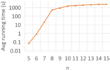
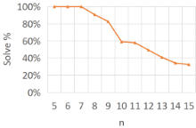
In order to evaluate the state-of-the-art integer counting techniques, we performed experiments with BARVINOK over random benchmarks (generated as described in Section 5). In Figures 1a and 1b we show the average running times and the percentages of benchmarks which BARVINOK was able to complete within one hour, with respect to the number of variables n. Note that the timeout is 3600s and there are some simple benchmarks for each n. Although the curve in Figure 1a appears to converge for n ≥ 9, with larger timeouts it
- (a) Average running time (b) Percentage solved instances.
Figure 1: Over different number of variables n.
would continue to increase. In general, the running time of BARVINOK seems to grow exponentially with increasing n. To reduce the number of variables, a rather straightforward idea is to decompose the constraints into components with a disjoint set of variables, which however is only possible if the dependencies graph between variables in the given constraints is also decomposable. Our goal is to extend such a decomposition technique to a larger class of problems.
The first effective exact model counter for SAT was RELSAT [Jr. and Pehoushek, 2000]. It identifies disconnected components dynamically as the underlying DPLL procedure attempts to extend a partial assignment. This technique is still considered state-of-the-art for model counters [Sang et al., 2004; Thurley, 2006; Sharma et al., 2019] and it inspired us to decompose linear constraints after assigning values to some variables. Note that each partial assignment corresponds to a counting sub-problem, so there may be thousands of subproblems. Fortunately, as the experiments described in Figures 1a and 1b indicate, it is possible that BARVINOK takes less time to compute thousands of smaller sub-problems than the original problem. So we propose to apply this idea of creating decomposable problems to improve integer counting.
3 Preliminaries
Definition 1. A linear constraint is an inequality of the form a1x1 + · · · + anxn op b, where xi are numeric variables, ai are constant coefficients, and op ∈ {<, ≤, >, ≥, =}.
Without loss of generality, a set of linear constraints with respect to the integer domain can be written in the form of: Ax ≤ b, where A is a m×n coefficient matrix and b is a 1×n constant vector. The m and n are the numbers of linear constraints and integer variables respectively. In the view of geometry, a linear constraint is a hyperplane in Euclidean space, and a set of linear constraints is an n-dimensional polytope. The number of integer models of the linear constraints is the same as the number of integer points inside the corresponding polytope. In this paper, we assume that the polytope contains only finite integer points, otherwise, there exists at least one integer variable with infinite domain, which can be easily detected via Integer Linear Programming (ILP). Note that in our experiments, the running time of ILP is negligible compared to that of the integer counting.
Definition 2. Given a set of constraints P = {Ax ≤ b}.
- Let #P denote the integer count in P.
- Let P[xi=c] represent the sub-problemwhere xi has been assigned the value c.
- Let RP denote the set of rows of P , where a row r ∈ RP corresponds to a constraint in P , as well as a row of A.
- Let CP denote the set of columns of P, where a column c ∈ CP corresponds to a variable of P, as well as a column of A.
- Let A[R,C] represent the sub-matrix of A that is generated by extracting rows R and columns C. Note that A[R, C] is an |R| × |C| matrix, and A = A[RP , CP ].
- Let b[R] and x[C] similarly represent the sub-vectors of b and x respectively.
- Let P[R,C] = {A[R,C]x[C] ≤ b[R]}. It is a subproblem of P that is generated by extracting rows R and columns C. Thus P [R, C] is a |C|-dimensional problem that consists of |R| linear constraints. In particular, we have P = P [RP , CP ].
Definition 3. The Linear Constraint Graph (LCG) of a set of linear constraints is constructed by the following rules:
- V = X, where X is the set of variables,
- for each pair of vertices (vi, vj), introduce an edge eij ∈ E and a weight wij on it, where wij equals the number of times that xi and xj appear together in a constraint.
4 Algorithm
Let P = {Ax ≤ b} be a set of constraints with matrix
Then P can be trivially decomposed into k sub-problems: {P1, . . . , Pk}, where Pi = Diγi ≤ βi, γi and βi are corresponding sub-vectors of x and b. Let #P and #Pi denote the integer counts in polytope P and Pi. Naturally, we have
To identify the sub-matrices Di in A, we introduce the Linear Constraint Graph (LCG) G(P) of P . If we remove edges with weight zero in the G(P), the different connected components (CCs) correspond to disjoint sets of variables.
Example 1. Consider a set of linear constraints
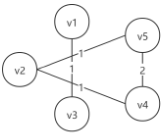
Figure 2 is the LCG of this problem. There are two connected components {v1, v3} and {v2, v4, v5} in this graph. They correspond to two sets of variables {x1, x3} and {x2, x4, x5} and two sets of constraints
This direct decomposition method requires special structures of matrix A, which limits its usage. The goal of this paper is to propose methods to create this kind of structure.
4.1 Column Elimination
When a variable is eliminated, the matrix A may turn into the form of Equation (1), and thus the problem can be decomposed. In our approach, we eliminate a variable by enumerating all its values and substituting it by that constant. Note the range of each integer variable xi should be finite and can be extracted through ILP. Assume xi ∈ [Li, Ui] = Xi, then
Note that P[xi=c] may be suitable for decomposition like Equation (1). Since eliminating a variable also causes the elimination of a column from A. Thus we call this process column elimination. This idea has already been used in #SAT [Jr. and Pehoushek, 2000], #CSP [Ganian et al., 2020], as well as counting linear extensions [Kangas et al., 2018], but not in counting linear constraints yet.
Given a set of linear constraints P = {Ax ≤ b} and assume the matrix A is in the form
Let s denote the width of Ei and
The column vectors γi and βi are the corresponding subvectors of x and b. Further note that γ0 = (x1, . . . , xs)T . Then after assigning values to γ0, P can be decomposed into k sub-problems:
where PCi(c) = Diγi ≤ βi - Eic. With Equation (3) we obtain the following theorem.
Theorem 1. #P = ∑c∈Γ0 ∏ki=1 #PCi(c), where Γ0 is the domain of γ0.
Consider the range Xi of variable xi in γ0. We know that Γ0 ⊆ X1×· · ·×Xs. However, since #PCi(c) = 0, for each c ∈ (X′1 × · · · ×X′s ) \ (X1 × · · · ×Xs), we further have the following corollary.
Corollary 1. #P = ∑c∈X1×···×Xs ∏ki=1 #PCi(c), where Xi is the range of variable xi in γ0.
We adopt Corollary 1 for convenience in our implementation. Note that in our implementation we check the satisfiability of PCi(c) (if the count is 0) when an assignment c is only partially assigned, to save computation.
4.2 Row Elimination
A row of the matrix A and vector b represents a linear constraint. Similar to our column elimination strategy, our new proposed row elimination strategy will also turn A into the form of Equation (1). However, the method to eliminate rows is more involved than eliminating columns. Without loss of generality, we assume that A has the form
Let t denote the height of Ei. Further, let
where γi and βi are the corresponding sub-vectors of x and b. Now we introduce (k - 1) × t new auxiliary variables
Let yi = (yi1, . . . yit)T = Eiγi, where 1 ≤ i ≤ k - 1. Then
If we assign values to the yi, then the problem can be decomposed into k sub-problems:
Since variables xi are bounded, yij are also bounded. So the upper and lower bounds of yij are finite numbers. Similar to the column elimination, we have the following results.
Theorem 2. #P = ∑c∈Y ∏ki=1 #PRi(c), where Y is the domain of (y11, . . . , y(k-1)t).
Algorithm 1: Row and Column Selection
- 1 Function SelectRowsAndColumns(P, DEPTH LIMIT,
- 10
SIZE LIMIT) 2 Compute a score for each element in DP = RP ∪ CP ; 3 Sort DP according to the score; 4 R0,C0 ← ∅, depth ←DEPTH LIMIT; 5 for each subset D ⊂DP s.t. |D| ≤ depth do 6 Let R and C denote the rows and columns in D respectively; 7 Q ← P [RP \R, CP \C]; 8 if CountCC (Q) > 1 and MaxCCSize(Q) ≤ SIZE LIMIT then 9 R0 ← R, C0 ← C, depth ← |D|; return R0, C0;Corollary 2. #P = ∑c∈Y11×···×Y(k-1)t ∏ki=1 #PRi(c), where Yij represents the range of yij.
Example 2. Consider a problem
Obviously, we can eliminate row x1 + · · · + xn ≤ 10 to apply decomposition on the remaining constraints. First we introduce a variable y to represent x1 + · · · + xk, where k = ⌊n/2⌋. Then the constraints are turned into
Note that the range for y is [-8k, 7k]. Finally, the constraints can be decomposed into two components with around n/2 variables each by assigning values in [-8k, 7k] to y.
4.3 Row and Column Selection
Now we consider the algorithm to identify the rows and columns to be eliminated. Algorithm 1 presents our framework of the row and column selection. The input consists of the problem P and two constant parameters, DEPTH LIMIT and SIZE LIMIT. Let DP denote the union of RP and CP . The algorithm first computes a heuristic score for each element in DP , and sorts them based on this score. Then it enumerates subsets of DP while minimizing the depth |D|. The loop updates the remaining constraints Q of P after removing rows and columns in D. If the LCG of the updated Q contains more than one CC and the sizes of each CC stays below the SIZE LIMIT, then a feasible selection has been found. In this case, the feasible selection is saved and depth updated (actually decreased). Finally, the algorithm picks the next subset D such that |D| ≤ depth according to the sequence of elements in DP . Note that depth starts from the input constant DEPTH LIMIT. It then monotonically decreases each time the algorithm finds a feasible selection. Note that the remaining search space is reduced by decreasing depth.
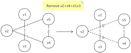
Incremental update of the LCG. Recall the definition of LCG, where a vertex corresponds to a variable, and the weight of an edge represents the number of constraints that contain both nodes (variables). When a row is removed (added), then for each pair of nodes that appear in this row, the LCG is updated by decreasing (increasing) the weight of the corresponding edge. Then the resulting graph is the LCG of the remaining constraints. Figure 3 demonstrates the update procedure for row removal on Example 1. When a column is removed, we simply remove the corresponding vertex. If the weight of an edge becomes zero the edge is considered to be removed. In this way, whenever a row or column is selected or deselected the LCG is updated incrementally.
4.4 Combining the Row and Column Eliminations
We already introduced a method which determines selected rows and columns in one pass. It is therefore natural to combine row and column eliminations in one single decomposition algorithm too. Without loss of generality, we assume matrix A to have the form
where the first t rows (F0,E1, . . . ,Ek) and s columns (F0, . . . , Fk) are selected to be eliminated. Further, let
where the γi and βi are the corresponding sub-vectors of x and b. Similar to the row elimination method, we first introduce (k - 1) × t new auxiliary variables {y11 . . . yk-1,t}. With yi = (yi1, . . . yit)T = Eiγi, we can transform P into
1 Function IntCount(P, DEPTH LIMIT, SIZE LIMIT) 2 C0,R0 ←SelectRowsAndColumns(P, DEPTH LIMIT, SIZE LIMIT); 3 s ← |C0|, t ← |R0|; 4 Q←P[RP\R0,CP\C0]; 5 (γ1, D1, β1), . . . , (γk, Dk, βk) ← FindAndMergeCC(Q, SIZE LIMIT); 6 β0, γ0,E1, . . . ,Ek, F0, . . . , Fk ←Process with R0, C0 and CCs; 7 Introduce variables yij , 1≤i≤k-1, 1≤j≤t; 8 Let yi = (yi1, . . . , yit)T ; 9 Pi← { Eiγi=yi Diγi≤βi-Fiγ0 , 1≤i≤k -1; 10 Pk← { Ekγk≤β0- ∑k-1 i=1 yi-F0γ0 Dkγk≤βk-Fkγ0 ; 11 for each xi ∈ γ0 do 12 Employ ILP to compute xi's bound Xi; 13 for each auxiliary variable yij do 14 Employ ILP to compute yij 's bound Yij ; 15 return ∑c∈X1×···×Xs×Y11×···×Y(k-1)t ∏ki=1 #Pi(c);If we assign values to γ0, y1, . . . , yk-1, then the problem can be decomposed into:
Finally, we have the following results.
Theorem 3. #P = ∑c∈D ∏ki=1 #Pi(c), where D is the domain of (x1, . . . , xs, y11, . . . , y(k-1)t).
Corollary 3. #P = ∑c∈X1×...×Xs×Y11×...×Y(k-1)t ∏ki=1 #Pi(c), where Xi represents the range of variable xi in γ0 and Yij represents the range of the auxiliary variable yij.
Our integer counting algorithm based on decomposition with column eliminations and row eliminations is presented in Algorithm 2. It first selects the columns and rows to be eliminated and obtains the remaining constraints Q. Then it determines all connected components (CCs) from the LCG of Q. These CCs correspond to different sets of variables γi, sub-matrices Di, and sub-vectors βi. Note that the number of introduced variables yij is closely related to the number of CCs. So the function "FindAndMergeCC" finds CCs first and then merges some of them in order to limit the size of CCs (to stay below SIZE LIMIT). Based on these CCs, the algorithm then obtains sub-matrices Ei and γ0 from Cols. After that, the problem P can be decomposed into k sub-problems Pk. Our approach employs ILP to obtain the bounds Xi and Yij.
Note that in our experiments, the running time of ILP is negligible compared to that of the integer counting subroutine. Finally, it applies Theorem 3 and calls integer counting subroutines to compute #Pi(c) for each assignment c from the domain X1 × · · · × Xs × Y11 × . . . Y(k-1)t and sums up.
5 Evaluation
Based on Algorithm 2, we implemented a prototype tool called INTCOUNT 1 in C++. Furthermore, we integrated INTCOUNT into a DPLL(T)-based #SMT(LA) counter [Ge et al., 2018]. We used a timeout of 3600 seconds, and chose SIZE LIMIT = ⌈n/2⌉. Another parameter DEPTH LIMIT was set to 4 if n ≥ 10, and 1 if n < 10. Experiments were conducted on Intel(R) Xeon(R) E5-2620 v4 @ 2.10GHz CPUs with a time limit of 3600 seconds and memory limit of 8 GB per benchmark. The benchmark set used in our experiments consists of two parts:
- Random Polytopes: We generated 2840 random benchmarks with three parameters (n,m, lmax), where n ∈ [5, 20] is the number of variables, m ∈ [1, n] is the number of constraints, and lmax ∈ [1, n] is the maximum length (non-zero coefficients) of constraints. The domain of variables is [-8, 7].
- Application Instances: We adopted 3953 benchmarks [Ge et al., 2019] from program analysis and simple temporal planning. Since most of the above program analysis benchmarks can be trivially handled by direct decomposition. We also generated 178 new and more challenging benchmarks by analyzing a Shell sort C program with less simplifications (modeling each element in an array and exploding a loop with more rounds). The domain of variables is [-32, 31].
We compared INTCOUNT with the state-of-the-art integer counter BARVINOK [Verdoolaege et al., 2007]. The tool BARVINOK is an exact integer counter for linear constraints and it is also used as the counting subroutine of our INTCOUNT. On random polytopes, we further compared our approach with the state-of-the-art propositional model counters like CACHET [Sang et al., 2004], GANAK [Sharma et al., 2019] and APPROXMC3 [Soos and Meel, 2019]. Note that they require CNF formulas as inputs. Thus we generated random polytopes not only with linear constraints, but also corresponding bit-vector formulas, which then were translated into propositional CNF with BOOLECTOR [Niemetz et al., 2018]. CNF translation time is not included in the running times of CACHET, GANAK and APPROXMC3. On application benchmarks, we only compared with BARVINOK. As they are all SMT(LA) formulas and we only integrated INTCOUNT and BARVINOK into a #SMT(LA) counter.
1 The source code and benchmarks can be found at "https:// github.com/bearben/intcount".
| Avg. selection search time | 0.0247 s |
| #Suitable for decomposition | 1916 (1180 solved, 736 timeouts) |
| #Direct call of BARVINOK | 924 (64 solved, 860 time- outs) |
| #Total benchmarks | 2840 (1244 solved, 1596 timeouts) |
| Avg. #sub-problems after de- composition | 1695 |
| Avg. size of sub-problems | ¯m = 8.202, ¯n = 3.011 |
| Avg. size of original problems | ¯m = 34.468, ¯n = 14.256 |
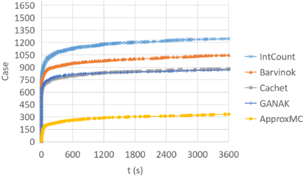
Figure 4 shows how many instances completed after a certain amount of time for INTCOUNT, BARVINOK, CACHET, GANAK and APPROXMC3. Clearly INTCOUNT can handle more cases than the other approaches. However, still more than half of the benchmarks cannot be handled in a reasonable time by any approaches. It indicates that there is a lot of room for improvements of integer counting algorithms.
Note that domain of variables in these benchmarks is rather small for BARVINOK. Moreover, in our algorithm, the variable domain size is directly related to the size of the Cartesian product of the components. Thus with increasing domain size our algorithm will become much less effective. By that time, INTCOUNT will give up decomposition and call BARVINOK on P directly instead. On the other hand, when domain size decreases, INTCOUNT will be more effective.
Table 1 summarizes the results of INTCOUNT over the random polytope benchmarks. The average running time of selection searching (Algorithm 1) is 0.0247s, which is usually negligible compared with the running time of counting subroutines. There are 1916 problems that can be decomposed by our approach. INTCOUNT solved 1180 of them. On these 1180 cases, Table 1 lists the average number of sub-problems (#calls of BARVINOK) for each problem, average size of all sub-problems and average size of these benchmarks. The results show that our decomposition techniques significantly reduce the size of problems for the counting subroutine.
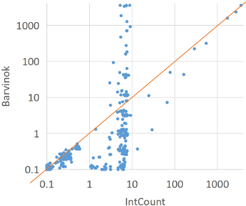
Figure 5 shows results on application benchmarks. The x-axis and y-axis are the running time of INTCOUNT and BARVINOK respectively. We observe that BARVINOK is superior on benchmarks that can be handled by BARVINOK in a few seconds, while INTCOUNT wins on benchmarks that cannot be handled by BARVINOK in 10s. Since after the decomposition, our approach sometimes has to solve a large number of sub-problems. Thus INTCOUNT may take more time. It suggests us implementing a computational cost estimation technique to determine if it is worth the decomposition. In general, the results show that our approach is useful for extending the capability of state-of-the-art integer counters.
6 RelatedWorks
There is a few related works which also utilize structural properties of problem instances for decomposition. Ganian et al. [Ganian et al., 2020] studied tree width and hyper-tree width of CSP problems, in order to exploit decomposability and guide dynamic programming methods for solving the problem. The definition of tree and hyper-tree shares the similar idea with column elimination in this paper. Tree nodes are the sub-problems after decomposition. Similar tree decomposition ideas are also used in algorithms for counting linear extensions [Kangas et al., 2018]. A linear extension of a partial order is a total order that is compatible with the given partial order. Finding linear extensions can be modeled by difference logic formulas, which is a special case of LC.
7 Conclusion
Motivated by decomposition techniques used in propositional model counting, this paper introduces novel column and row elimination techniques which allow to decompose integer counting problems for linear constraints into independent sub-problems. Our experiments on an extensive set of benchmarks show that our algorithm improves performance of the state-of-the-art integer counting tools while the overhead for finding decomposition is negligible. At this point, domain size is still a limiting factor in our approach and we intend to overcome this hurdle in the future.
Acknowledgments
This work is supported the Linz Institute of Technology (LIT) AI Lab funded by the State of Upper Austria.
@inproceedings{ijcai2021p192,
  title     = {Decomposition Strategies to Count Integer Solutions over Linear Constraints},
  author    = {Ge, Cunjing and Biere, Armin},
  booktitle = {Proceedings of the Thirtieth International Joint Conference on
               Artificial Intelligence, {IJCAI-21}},
  publisher = {International Joint Conferences on Artificial Intelligence Organization},
  editor    = {Zhi-Hua Zhou},
  pages     = {1389--1395},
  year      = {2021},
  month     = {8},
  note      = {Main Track},
  doi       = {10.24963/ijcai.2021/192},
  url       = {https://doi.org/10.24963/ijcai.2021/192},
}
TY - CPAPER TI - Decomposition Strategies to Count Integer Solutions over Linear Constraints AU - Ge, Cunjing AU - Biere, Armin T2 - Proceedings of the Thirtieth International Joint Conference on Artificial Intelligence, IJCAI-21 PB - International Joint Conferences on Artificial Intelligence Organization PY - 2021 SP - 1389 EP - 1395 DO - 10.24963/ijcai.2021/192 UR - https://doi.org/10.24963/ijcai.2021/192 ER -Copied
Machine-readable versions of this paper, for tools and AI agents:





